This function compute the global spatial runs test for spatial independence of a categorical spatial data set.
Usage
sp.runs.test(formula = NULL, data = NULL, fx = NULL,
listw = listw, alternative = "two.sided" ,
distr = "asymptotic", nsim = NULL,control = list())
Arguments
- formula
a symbolic description of the factor (optional).
- data
an (optional) data frame or a sf object containing the variable to testing for.
- fx
a factor (optional).
- listw
A neighbourhood list (type knn or nb) or a W matrix that indicates the order of the elements in each \(m_i-environment\) (for example of inverse distance). To calculate the number of runs in each \(m_i-environment\), an order must be established, for example from the nearest neighbour to the furthest one.
- alternative
a character string specifying the alternative hypothesis, must be one of "two.sided" (default), "greater" or "less".
- distr
A string. Distribution of the test "asymptotic" (default) or "bootstrap".
- nsim
Number of permutations to obtain pseudo-value and confidence intervals (CI). Default value is NULL to don`t get CI of number of runs.
- control
List of additional control arguments.
Value
A object of the htest and sprunstest class
data.name | a character string giving the names of the data. |
method | the type of test applied (). |
SR | total number of runs |
dnr | empirical distribution of the number of runs |
statistic | Value of the homogeneity runs statistic. Negative sign indicates global homogeneity |
alternative | a character string describing the alternative hypothesis. |
p.value | p-value of the SRQ |
pseudo.value | the pseudo p-value of the SRQ test if nsim is not NULL |
MeanNeig | Mean of the Maximum number of neighborhood |
MaxNeig | Maximum number of neighborhood |
listw | The list of neighborhood |
nsim | number of boots (only for boots version) |
SRGP | nsim simulated values of statistic. |
SRLP | matrix with the number of runs for eacl localization. |
Details
The order of the neighbourhoods (\(m_i-environments\)) is critical to obtain the test.
To obtain the number of runs observed in each \(m_i-environment\), each element must be associated
with a set of neighbours ordered by proximity.
Three kinds of lists can be included to identify \(m_i-environments\):
knn: Objects of the class knn that consider the neighbours in order of proximity.nb: If the neighbours are obtained from an sf object, the code internally will call the functionnb2nb_orderit will order them in order of proximity of the centroids.matrix: If a object of matrix class based in the inverse of the distance in introduced as argument, the functionnb2nb_orderwill also be called internally to transform the object the class matrix to a matrix of the class nb with ordered neighbours.
Two alternative sets of arguments can be included in this function to compute the spatial runs test:
Option 1 | A factor (fx) and a list of neighborhood (listw) of the class knn. |
Option 2 | A sf object (data) and formula to specify the factor. A list of neighbourhood (listw) |
Definition of spatial run
In this section define the concepts of spatial encoding and runs, and construct the main statistics necessary
for testing spatial homogeneity of categorical variables. In order to develop a general theoretical setting,
let us consider \(\{X_s\}_{s \in S}\) to be the categorical spatial process of interest with Q different
categories, where S is a set of coordinates.
Spatial encoding:
For a location \(s \in S\) denote by \(N_s = \{s_1,s_2 ...,s_{n_s}\}\) the set of neighbours according
to the interaction scheme W, which are ordered from lesser to higher Euclidean distance with respect to location s.
The sequence as \(X_{s_i} , X_{s_i+1},...,, X_{s_i+r}\) its elements have the same value (or are identified by the same class)
is called a spatial run at location s of length r.
Spatial run statistic
The total number of runs is defined as:
$$SR^Q=n+\sum_{s \in S}\sum_{j=1}^{n_s}I_j^s$$
where \(I_j^s = 1 \ if \ X_{s_j-1} \neq X_{s_j} \ and 0 \ otherwise\) for \(j=1,2,...,n_s\)
Following result by the Central Limit Theorem, the asymtotical distribution of \(SR^Q\) is:
$$SR^Q = N(\mu_{SR^Q},\sigma_{SR^Q})$$
In the one-tailed case, we must distinguish the lower-tailed test and the upper-tailed, which are associated
with homogeneity and heterogeneity respectively. In the case of the lower-tailed test,
the following hypotheses are used:
\(H_0:\{X_s\}_{s \in S}\) is i.i.d.
\(H_1\): The spatial distribution of the values of the categorical variable is more homogeneous than under the null hypothesis (according to the fixed association scheme).
In the upper-tailed test, the following hypotheses are used:
\(H_0:\{X_s\}_{s \in S}\) is i.i.d.
\(H_1\): The spatial distribution of the values of the categorical variable is more
heterogeneous than under the null hypothesis (according to the fixed association scheme).
These hypotheses provide a decision rule regarding the degree of homogeneity in the spatial distribution
of the values of the spatial categorical random variable.
Control arguments
seedinit | Numerical value for the seed (only for boot version). Default value seedinit=123 |
References
Ruiz, M., López, F., and Páez, A. (2021). A test for global and local homogeneity of categorical data based on spatial runs. Working paper.
Author
| Fernando López | fernando.lopez@upct.es |
| Román Mínguez | roman.minguez@uclm.es |
| Antonio Páez | paezha@gmail.com |
| Manuel Ruiz | manuel.ruiz@upct.es |
Examples
# Case 1: SRQ test based on factor and knn
# \donttest{
n <- 100
cx <- runif(n)
cy <- runif(n)
x <- cbind(cx,cy)
listw <- spdep::knearneigh(cbind(cx,cy), k=3)
p <- c(1/6,3/6,2/6)
rho <- 0.5
fx <- dgp.spq(listw = listw, p = p, rho = rho)
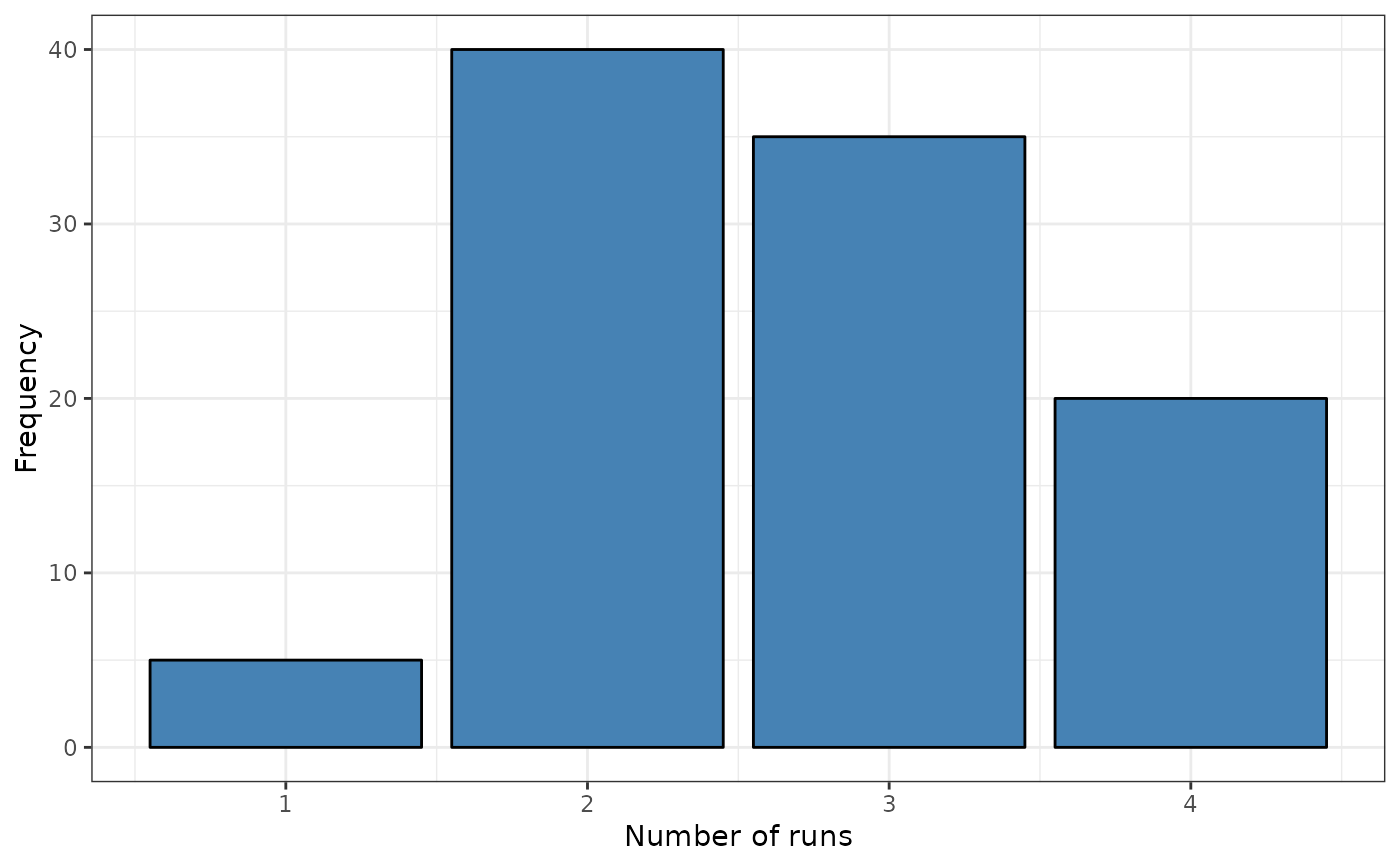
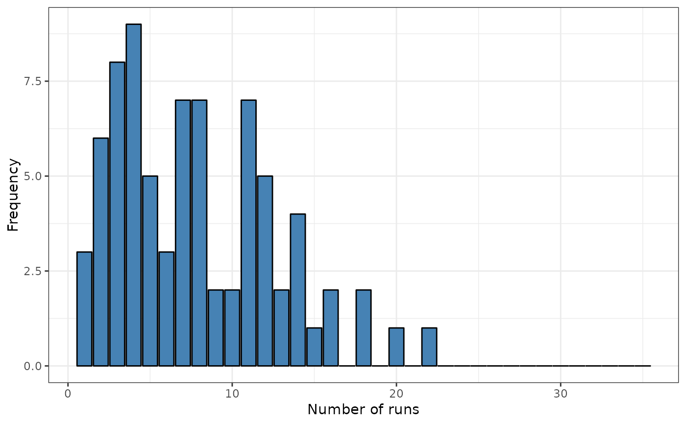
srq <- sp.runs.test(fx = fx, listw = listw)
print(srq)
#>
#> Runs test of spatial dependence for qualitative data. Asymptotic
#> version
#>
#> data: mxf
#> sp.runs test = -1.0212, p-value = 0.3072
#> alternative hypothesis: two.sided
#> sample estimates:
#> Total runs Mean total runs Variance total runs
#> 274.0000 285.5152 127.1573
#>
plot(srq)
 # Boots Version
control <- list(seedinit = 1255)
srq <- sp.runs.test(fx = fx, listw = listw, distr = "bootstrap" , nsim = 299, control = control)
print(srq)
#>
#> Runs test of spatial dependence for qualitative data. Boots version
#>
#> data: mxf
#> sp.runs test = -1.0212, p-value = 0.28
#> alternative hypothesis: two.sided
#> sample estimates:
#> Observed Total runs Mean total runs boots Variance total runs boots
#> 274.0000 285.8662 131.4518
#>
plot(srq)
# Boots Version
control <- list(seedinit = 1255)
srq <- sp.runs.test(fx = fx, listw = listw, distr = "bootstrap" , nsim = 299, control = control)
print(srq)
#>
#> Runs test of spatial dependence for qualitative data. Boots version
#>
#> data: mxf
#> sp.runs test = -1.0212, p-value = 0.28
#> alternative hypothesis: two.sided
#> sample estimates:
#> Observed Total runs Mean total runs boots Variance total runs boots
#> 274.0000 285.8662 131.4518
#>
plot(srq)
 # Case 2: SRQ test with formula, a sf object (points) and knn
data("FastFood.sf")
x <- sf::st_coordinates(sf::st_centroid(FastFood.sf))
listw <- spdep::knearneigh(x, k=4)
formula <- ~ Type
srq <- sp.runs.test(formula = formula, data = FastFood.sf, listw = listw)
print(srq)
#>
#> Runs test of spatial dependence for qualitative data. Asymptotic
#> version
#>
#> data: Type
#> sp.runs test = 3.899, p-value = 9.657e-05
#> alternative hypothesis: two.sided
#> sample estimates:
#> Total runs Mean total runs Variance total runs
#> 3408.000 3216.242 2418.743
#>
plot(srq)
# Case 2: SRQ test with formula, a sf object (points) and knn
data("FastFood.sf")
x <- sf::st_coordinates(sf::st_centroid(FastFood.sf))
listw <- spdep::knearneigh(x, k=4)
formula <- ~ Type
srq <- sp.runs.test(formula = formula, data = FastFood.sf, listw = listw)
print(srq)
#>
#> Runs test of spatial dependence for qualitative data. Asymptotic
#> version
#>
#> data: Type
#> sp.runs test = 3.899, p-value = 9.657e-05
#> alternative hypothesis: two.sided
#> sample estimates:
#> Total runs Mean total runs Variance total runs
#> 3408.000 3216.242 2418.743
#>
plot(srq)
 # Version boots
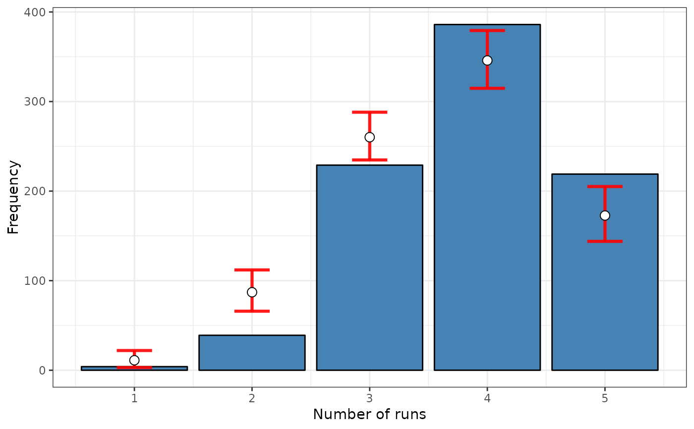
srq <- sp.runs.test(formula = formula, data = FastFood.sf, listw = listw,
distr = "bootstrap", nsim = 199)
print(srq)
#>
#> Runs test of spatial dependence for qualitative data. Boots version
#>
#> data: Type
#> sp.runs test = 3.899, p-value < 2.2e-16
#> alternative hypothesis: two.sided
#> sample estimates:
#> Observed Total runs Mean total runs boots Variance total runs boots
#> 3408.000 3213.030 2597.191
#>
plot(srq)
# Version boots
srq <- sp.runs.test(formula = formula, data = FastFood.sf, listw = listw,
distr = "bootstrap", nsim = 199)
print(srq)
#>
#> Runs test of spatial dependence for qualitative data. Boots version
#>
#> data: Type
#> sp.runs test = 3.899, p-value < 2.2e-16
#> alternative hypothesis: two.sided
#> sample estimates:
#> Observed Total runs Mean total runs boots Variance total runs boots
#> 3408.000 3213.030 2597.191
#>
plot(srq)
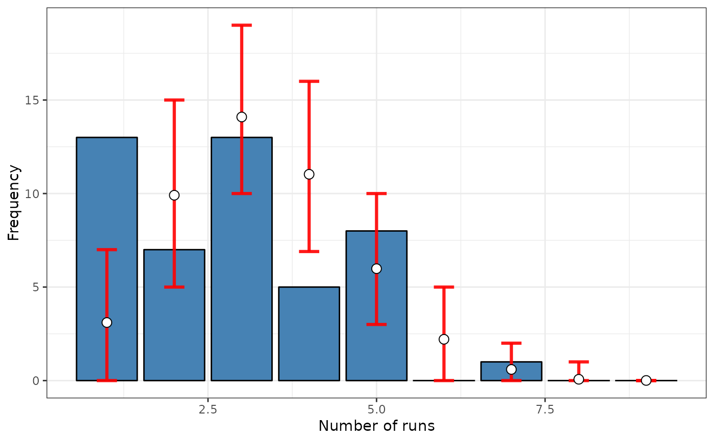
 # Case 3: SRQ test (permutation) using formula with a sf object (polygons) and nb
library(sf)
fname <- system.file("shape/nc.shp", package="sf")
nc <- sf::st_read(fname)
#> Reading layer `nc' from data source
#> `/home/runner/work/_temp/Library/sf/shape/nc.shp' using driver `ESRI Shapefile'
#> Simple feature collection with 100 features and 14 fields
#> Geometry type: MULTIPOLYGON
#> Dimension: XY
#> Bounding box: xmin: -84.32385 ymin: 33.88199 xmax: -75.45698 ymax: 36.58965
#> Geodetic CRS: NAD27
listw <- spdep::poly2nb(as(nc,"Spatial"), queen = FALSE)
#> although coordinates are longitude/latitude, st_intersects assumes that they
#> are planar
p <- c(1/6,3/6,2/6)
rho = 0.5
co <- sf::st_coordinates(sf::st_centroid(nc))
#> Warning: st_centroid assumes attributes are constant over geometries
#> Warning: st_centroid does not give correct centroids for longitude/latitude data
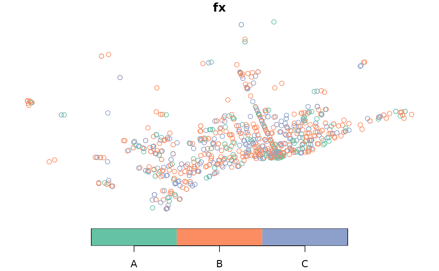
nc$fx <- dgp.spq(listw = listw, p = p, rho = rho)
plot(nc["fx"])
# Case 3: SRQ test (permutation) using formula with a sf object (polygons) and nb
library(sf)
fname <- system.file("shape/nc.shp", package="sf")
nc <- sf::st_read(fname)
#> Reading layer `nc' from data source
#> `/home/runner/work/_temp/Library/sf/shape/nc.shp' using driver `ESRI Shapefile'
#> Simple feature collection with 100 features and 14 fields
#> Geometry type: MULTIPOLYGON
#> Dimension: XY
#> Bounding box: xmin: -84.32385 ymin: 33.88199 xmax: -75.45698 ymax: 36.58965
#> Geodetic CRS: NAD27
listw <- spdep::poly2nb(as(nc,"Spatial"), queen = FALSE)
#> although coordinates are longitude/latitude, st_intersects assumes that they
#> are planar
p <- c(1/6,3/6,2/6)
rho = 0.5
co <- sf::st_coordinates(sf::st_centroid(nc))
#> Warning: st_centroid assumes attributes are constant over geometries
#> Warning: st_centroid does not give correct centroids for longitude/latitude data
nc$fx <- dgp.spq(listw = listw, p = p, rho = rho)
plot(nc["fx"])
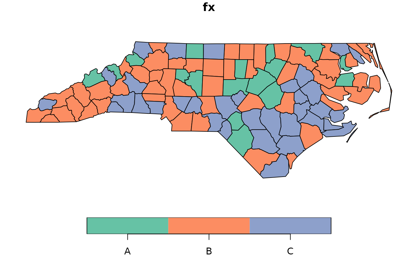 formula <- ~ fx
srq <- sp.runs.test(formula = formula, data = nc, listw = listw,
distr = "bootstrap", nsim = 399)
#> Warning: st_centroid assumes attributes are constant over geometries
#> Warning: st_centroid does not give correct centroids for longitude/latitude data
print(srq)
#>
#> Runs test of spatial dependence for qualitative data. Boots version
#>
#> data: fx
#> sp.runs test = -1.2198, p-value = 0.2025
#> alternative hypothesis: two.sided
#> sample estimates:
#> Observed Total runs Mean total runs boots Variance total runs boots
#> 371.0000 386.3609 138.9046
#>
plot(srq)
formula <- ~ fx
srq <- sp.runs.test(formula = formula, data = nc, listw = listw,
distr = "bootstrap", nsim = 399)
#> Warning: st_centroid assumes attributes are constant over geometries
#> Warning: st_centroid does not give correct centroids for longitude/latitude data
print(srq)
#>
#> Runs test of spatial dependence for qualitative data. Boots version
#>
#> data: fx
#> sp.runs test = -1.2198, p-value = 0.2025
#> alternative hypothesis: two.sided
#> sample estimates:
#> Observed Total runs Mean total runs boots Variance total runs boots
#> 371.0000 386.3609 138.9046
#>
plot(srq)
 # Case 4: SRQ test (Asymptotic) using formula with a sf object (polygons) and nb
data(provinces_spain)
# sf::sf_use_s2(FALSE)
listw <- spdep::poly2nb(provinces_spain, queen = FALSE)
#> although coordinates are longitude/latitude, st_intersects assumes that they
#> are planar
#> Warning: some observations have no neighbours;
#> if this seems unexpected, try increasing the snap argument.
#> Warning: neighbour object has 4 sub-graphs;
#> if this sub-graph count seems unexpected, try increasing the snap argument.
provinces_spain$Coast <- factor(provinces_spain$Coast)
levels(provinces_spain$Coast) = c("no","yes")
plot(provinces_spain["Coast"])
# Case 4: SRQ test (Asymptotic) using formula with a sf object (polygons) and nb
data(provinces_spain)
# sf::sf_use_s2(FALSE)
listw <- spdep::poly2nb(provinces_spain, queen = FALSE)
#> although coordinates are longitude/latitude, st_intersects assumes that they
#> are planar
#> Warning: some observations have no neighbours;
#> if this seems unexpected, try increasing the snap argument.
#> Warning: neighbour object has 4 sub-graphs;
#> if this sub-graph count seems unexpected, try increasing the snap argument.
provinces_spain$Coast <- factor(provinces_spain$Coast)
levels(provinces_spain$Coast) = c("no","yes")
plot(provinces_spain["Coast"])
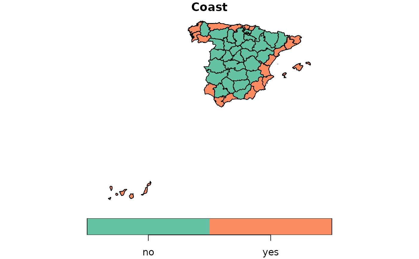 formula <- ~ Coast
srq <- sp.runs.test(formula = formula, data = provinces_spain, listw = listw)
#> Warning: st_centroid assumes attributes are constant over geometries
#> Warning: st_centroid does not give correct centroids for longitude/latitude data
print(srq)
#>
#> Runs test of spatial dependence for qualitative data. Asymptotic
#> version
#>
#> data: Coast
#> sp.runs test = -2.7795, p-value = 0.005444
#> alternative hypothesis: two.sided
#> sample estimates:
#> Total runs Mean total runs Variance total runs
#> 133.00000 160.36571 96.93415
#>
plot(srq)
formula <- ~ Coast
srq <- sp.runs.test(formula = formula, data = provinces_spain, listw = listw)
#> Warning: st_centroid assumes attributes are constant over geometries
#> Warning: st_centroid does not give correct centroids for longitude/latitude data
print(srq)
#>
#> Runs test of spatial dependence for qualitative data. Asymptotic
#> version
#>
#> data: Coast
#> sp.runs test = -2.7795, p-value = 0.005444
#> alternative hypothesis: two.sided
#> sample estimates:
#> Total runs Mean total runs Variance total runs
#> 133.00000 160.36571 96.93415
#>
plot(srq)
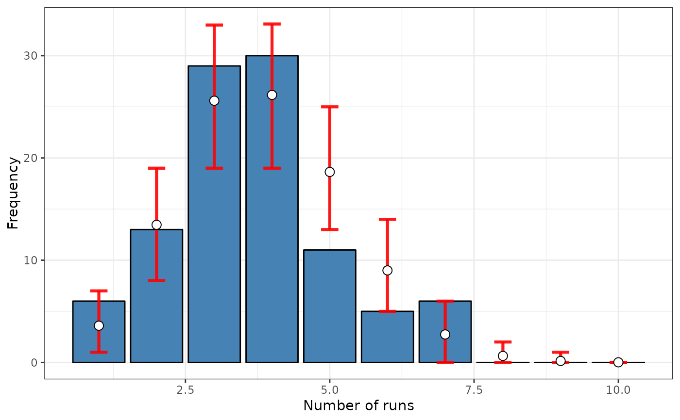
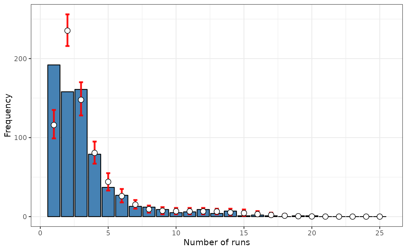
 # Boots version
srq <- sp.runs.test(formula = formula, data = provinces_spain, listw = listw,
distr = "bootstrap", nsim = 299)
#> Warning: st_centroid assumes attributes are constant over geometries
#> Warning: st_centroid does not give correct centroids for longitude/latitude data
print(srq)
#>
#> Runs test of spatial dependence for qualitative data. Boots version
#>
#> data: Coast
#> sp.runs test = -2.7795, p-value = 0.003333
#> alternative hypothesis: two.sided
#> sample estimates:
#> Observed Total runs Mean total runs boots Variance total runs boots
#> 133.00000 157.27425 92.83058
#>
plot(srq)
# Boots version
srq <- sp.runs.test(formula = formula, data = provinces_spain, listw = listw,
distr = "bootstrap", nsim = 299)
#> Warning: st_centroid assumes attributes are constant over geometries
#> Warning: st_centroid does not give correct centroids for longitude/latitude data
print(srq)
#>
#> Runs test of spatial dependence for qualitative data. Boots version
#>
#> data: Coast
#> sp.runs test = -2.7795, p-value = 0.003333
#> alternative hypothesis: two.sided
#> sample estimates:
#> Observed Total runs Mean total runs boots Variance total runs boots
#> 133.00000 157.27425 92.83058
#>
plot(srq)
 # Case 5: SRQ test based on a distance matrix (inverse distance)
N <- 100
cx <- runif(N)
cy <- runif(N)
data <- as.data.frame(cbind(cx,cy))
data <- sf::st_as_sf(data,coords = c("cx","cy"))
n = dim(data)[1]
dis <- 1/matrix(as.numeric(sf::st_distance(data,data)),ncol=n,nrow=n)
diag(dis) <- 0
dis <- (dis < quantile(dis,.10))*dis
p <- c(1/6,3/6,2/6)
rho <- 0.5
fx <- dgp.spq(listw = dis , p = p, rho = rho)
srq <- sp.runs.test(fx = fx, listw = dis)
print(srq)
#>
#> Runs test of spatial dependence for qualitative data. Asymptotic
#> version
#>
#> data: mxf
#> sp.runs test = 0.039001, p-value = 0.9689
#> alternative hypothesis: two.sided
#> sample estimates:
#> Total runs Mean total runs Variance total runs
#> 658.0000 656.5455 1390.9461
#>
plot(srq)
# Case 5: SRQ test based on a distance matrix (inverse distance)
N <- 100
cx <- runif(N)
cy <- runif(N)
data <- as.data.frame(cbind(cx,cy))
data <- sf::st_as_sf(data,coords = c("cx","cy"))
n = dim(data)[1]
dis <- 1/matrix(as.numeric(sf::st_distance(data,data)),ncol=n,nrow=n)
diag(dis) <- 0
dis <- (dis < quantile(dis,.10))*dis
p <- c(1/6,3/6,2/6)
rho <- 0.5
fx <- dgp.spq(listw = dis , p = p, rho = rho)
srq <- sp.runs.test(fx = fx, listw = dis)
print(srq)
#>
#> Runs test of spatial dependence for qualitative data. Asymptotic
#> version
#>
#> data: mxf
#> sp.runs test = 0.039001, p-value = 0.9689
#> alternative hypothesis: two.sided
#> sample estimates:
#> Total runs Mean total runs Variance total runs
#> 658.0000 656.5455 1390.9461
#>
plot(srq)
 srq <- sp.runs.test(fx = fx, listw = dis, data = data)
#> Warning: style is M (missing); style should be set to a valid value
#> Warning: no-neighbour observations found, set zero.policy to TRUE;
#> this warning will soon become an error
#> Warning: neighbour object has 24 sub-graphs
print(srq)
#>
#> Runs test of spatial dependence for qualitative data. Asymptotic
#> version
#>
#> data: mxf
#> sp.runs test = 0.039001, p-value = 0.9689
#> alternative hypothesis: two.sided
#> sample estimates:
#> Total runs Mean total runs Variance total runs
#> 658.0000 656.5455 1390.9461
#>
plot(srq)
srq <- sp.runs.test(fx = fx, listw = dis, data = data)
#> Warning: style is M (missing); style should be set to a valid value
#> Warning: no-neighbour observations found, set zero.policy to TRUE;
#> this warning will soon become an error
#> Warning: neighbour object has 24 sub-graphs
print(srq)
#>
#> Runs test of spatial dependence for qualitative data. Asymptotic
#> version
#>
#> data: mxf
#> sp.runs test = 0.039001, p-value = 0.9689
#> alternative hypothesis: two.sided
#> sample estimates:
#> Total runs Mean total runs Variance total runs
#> 658.0000 656.5455 1390.9461
#>
plot(srq)
 # Boots version
srq <- sp.runs.test(fx = fx, listw = dis, data = data, distr = "bootstrap", nsim = 299)
#> Warning: style is M (missing); style should be set to a valid value
#> Warning: no-neighbour observations found, set zero.policy to TRUE;
#> this warning will soon become an error
#> Warning: neighbour object has 24 sub-graphs
print(srq)
#>
#> Runs test of spatial dependence for qualitative data. Boots version
#>
#> data: mxf
#> sp.runs test = 0.039001, p-value = 0.9833
#> alternative hypothesis: two.sided
#> sample estimates:
#> Observed Total runs Mean total runs boots Variance total runs boots
#> 658.0000 632.3244 1430.1259
#>
plot(srq)
# Boots version
srq <- sp.runs.test(fx = fx, listw = dis, data = data, distr = "bootstrap", nsim = 299)
#> Warning: style is M (missing); style should be set to a valid value
#> Warning: no-neighbour observations found, set zero.policy to TRUE;
#> this warning will soon become an error
#> Warning: neighbour object has 24 sub-graphs
print(srq)
#>
#> Runs test of spatial dependence for qualitative data. Boots version
#>
#> data: mxf
#> sp.runs test = 0.039001, p-value = 0.9833
#> alternative hypothesis: two.sided
#> sample estimates:
#> Observed Total runs Mean total runs boots Variance total runs boots
#> 658.0000 632.3244 1430.1259
#>
plot(srq)
 # Case 6: SRQ test based on a distance matrix (inverse distance)
data("FastFood.sf")
# sf::sf_use_s2(FALSE)
n = dim(FastFood.sf)[1]
dis <- 1000000/matrix(as.numeric(sf::st_distance(FastFood.sf,FastFood.sf)), ncol = n, nrow = n)
diag(dis) <- 0
dis <- (dis < quantile(dis,.005))*dis
p <- c(1/6,3/6,2/6)
rho = 0.5
co <- sf::st_coordinates(sf::st_centroid(FastFood.sf))
FastFood.sf$fx <- dgp.spq(p = p, listw = dis, rho = rho)
plot(FastFood.sf["fx"])
# Case 6: SRQ test based on a distance matrix (inverse distance)
data("FastFood.sf")
# sf::sf_use_s2(FALSE)
n = dim(FastFood.sf)[1]
dis <- 1000000/matrix(as.numeric(sf::st_distance(FastFood.sf,FastFood.sf)), ncol = n, nrow = n)
diag(dis) <- 0
dis <- (dis < quantile(dis,.005))*dis
p <- c(1/6,3/6,2/6)
rho = 0.5
co <- sf::st_coordinates(sf::st_centroid(FastFood.sf))
FastFood.sf$fx <- dgp.spq(p = p, listw = dis, rho = rho)
plot(FastFood.sf["fx"])
 formula <- ~ fx
# Boots version
srq <- sp.runs.test(formula = formula, data = FastFood.sf, listw = dis,
distr = "bootstrap", nsim = 299)
#> Warning: style is M (missing); style should be set to a valid value
#> Warning: no-neighbour observations found, set zero.policy to TRUE;
#> this warning will soon become an error
#> Warning: neighbour object has 650 sub-graphs
print(srq)
#>
#> Runs test of spatial dependence for qualitative data. Boots version
#>
#> data: fx
#> sp.runs test = -6.881, p-value = 0.003333
#> alternative hypothesis: two.sided
#> sample estimates:
#> Observed Total runs Mean total runs boots Variance total runs boots
#> 1657.000 2050.428 21820.937
#>
plot(srq)
formula <- ~ fx
# Boots version
srq <- sp.runs.test(formula = formula, data = FastFood.sf, listw = dis,
distr = "bootstrap", nsim = 299)
#> Warning: style is M (missing); style should be set to a valid value
#> Warning: no-neighbour observations found, set zero.policy to TRUE;
#> this warning will soon become an error
#> Warning: neighbour object has 650 sub-graphs
print(srq)
#>
#> Runs test of spatial dependence for qualitative data. Boots version
#>
#> data: fx
#> sp.runs test = -6.881, p-value = 0.003333
#> alternative hypothesis: two.sided
#> sample estimates:
#> Observed Total runs Mean total runs boots Variance total runs boots
#> 1657.000 2050.428 21820.937
#>
plot(srq)
 # }
# }