A function to compute Q test for spatial qualitative data.
Usage
Q.test(formula = NULL, data = NULL, na.action,
fx = NULL, coor = NULL, m = 3, r = 1, distr = "asymptotic",
control = list())
Arguments
- formula
a symbolic description of the factor(s).
- data
an (optional) data frame or a sf object with points/multipolygons geometry containing the variable(s) to be tested.
- na.action
action with NA values
- fx
a factor or a matrix of factors in columns
- coor
(optional) a 2xN vector with spatial coordinates. Used when data is not a spatial object
- m
length of m-surrounding (default = 3).
- r
only for asimtotic distribution. Maximum overlapping between any two m-surroundings (default = 1).
- distr
character. Distribution type "asymptotic" (default) or "mc".
- control
Optional argument. See Control Argument section.
Value
An list of two object of the class htest. Each element of the list return the:
data.name | a character string giving the names of the data. |
statistic | Value of the Q test |
N | total number of observations. |
R | total number of symbolized observations. |
m | length m-surrounding. |
r | degree of overlapping. |
df | degree of freedom. |
distr | type of distribution used to get the significance of the Q test. |
type | type of symbols. |
Details
The Q-test is a simple, consistent, and powerful statistic for qualitative spatial
independence that we develop using concepts from symbolic dynamics and symbolic
entropy. The Q test can be used to detect, given a spatial distribution of events,
patterns of spatial association of qualitative variables in a wide variety of
settings.
The Q(m) statistic was introduced by Ruiz et al. (2010) as a tool to explore geographical
co-location/co-occurrence of qualitative data. Consider a spatial variable X which is the
result of a qualitative process with a set number of categorical outcomes \(a_j\) (j=1,...,k).
The spatial variable is observed at a set of fixed locations indexed by their coordinates
\(s_i\) (i=1,..., N), so that at each location si where an event is observed,
\(X_i\) takes one of the possible values \(a_j\).
Since the observations are georeferenced, a spatial embedding protocol can be devised
to assess the spatial property of co-location. Let us define, for an observation at
a specified location, say \(s_0\), a surrounding of size m, called an m-surrounding.
The m-surrounding is the set of m-1 nearest neighbours from the perspective
of location \(s_0\). In the case of distance ties, a secondary criterion can be
invoked based on direction.
Once that an embedding protocol is adopted and the elements of the m-surrounding
for location \(s_0\) have been determined, a string can be obtained that collects
the elements of the local neighborhood (the m-1 nearest neighbors) of the observation
at \(s_0\). The m-surrounding can then be represented in the following way:
$$X_m(s_0)=(X_{s_0},X_{s_1},...X_{s_{m-1}})$$
Since each observation Xs takes one of k possible values, and there are m observations in
the m-surrounding, there are exactly k possible unique ways in which those values can
co-locate. This is the number of permutations with replacement.
For instance, if k=2
(e.g. the possible outcomes are a1=0 and a2=1) and m=3, the following eight unique
patterns of co-location are possible (the number of symbols is \(n_{\sigma}\)=8): (0,0,0), (1,0,0),
(0,1,0), (0,0,1), (1,1,0), (1,0,1), (0,1,1), and (1,1,1). Each unique co-locationtype
can be denoted in a convenient way by means of a symbol \(\sigma_i\) \((i=1, 2,...,k^m)\). It follows
that each site can be uniquely associated with a specific symbol, in a process termed
symbolization. In this way, we say that a location s is of type \(\sigma_i\) if and only if \(X_m(s)=\sigma_i\).
Equivalent symbols (see Páez, et al. 2012) can be obtained by counting the number of
occurrences of each category within an m-surrounding. This surrenders some
topological information (ordering within the m-surrounding is lost) in favor of a more
compact set of symbols, since the number of combinations with replacement.
Definition of Q(m) statistic
Let \(\{X_s\}_{s \in R}\) be a discrete spatial process and m be a fixed embedding
dimension. The statistic Q testing the null hypothesis:
\(H_0:\{X_s\}_{s \in R}\) is spatially independent, against any other alternative.
For a fixed \(m \geq 2\), the relative frequency of symbols can be used to define the symbolic
entropy of the spatial process as the Shanon entropy of the distinct symbols:
$$h(m) = - \sum_j p_{\sigma_j}ln(p_{\sigma_j})$$
where
$$p_{\sigma_j}={ n_{\sigma_j} \over R}$$
with \(n_{\sigma_j}\) is simply the
number of times that the symbol \(\sigma_j\) is observed and R the number of
symbolized locations.
The entropy function is bounded between \(0 < h (m) \leq \eta\).
The Q statistic is essentially a likelihood ratio test between the symbolic entropy
of the observed pattern and the entropy of the system under the null hypothesis
of a random spatial sequence:
$$Q(m)=2R(\eta-h(m))$$
with \(\eta = ln(k^m)\). The statistic is asymptotically \(\chi^2\) distributed
with degrees of freedom equal to the number of symbols minus one.
Control arguments
- distance
character to select the type of distance. Default = "Euclidean" for Cartesian coordinates only: one of Euclidean, Hausdorff or Frechet; for geodetic coordinates, great circle distances are computed (see sf::st_distance())
- dtmaxabs
Delete degenerate surrounding based on the absolute distance between observations.
- dtmaxpc
A value between 0 and 1. Delete degenerate surrounding based on the distance. Delete m-surrounding when the maximum distance between observation is upper than k percentage of maximum distance between anywhere observation.
- dtmaxknn
A integer value 'k'. Delete degenerate surrounding based on the near neighbourhood criteria. Delete m-surrounding is a element of the m-surrounding is not include in the set of k near neighbourhood of the first element
- nsim
number of simulations for get the Monte Carlo distribution. Default = 999
- seedinit
seed to select the initial element to star the algorithm to get compute the m-surroundings or to start the simulation
Standard-Permutation vs Equivalent-Combination Symbols
The symbolization protocol proposed by Ruiz et al. (2010) - call these
Standard-Permutation Symbols — contains a large amount of topological information
regarding the units of analysis, including proximity and direction.
In this sense, the protocol is fairly general. On the other hand, it is easy to see
that the combinatorial possibilities can very quickly become unmanageable.
For a process with k = 3 outcomes and m = 5, the number of symbols becomes
\(3^5 = 243\); for k = 6 and m = 4 it is \(6^4 = 1,296\). Depending on the number
of observations N, the explosion in the number of symbols can very rapidly consume
degrees of freedom for hypothesis testing, because as a rule of thumb
it is recommended that the number of symbolized locations be at least five times
the number of symbols used (e.g., \(R \geq 5k^m\)), and R will usually be a fraction of N.
As an alternative, we propose a symbolization protocol that sacrifices
some amount of topological detail for conciseness. The alternative is based
on the standard scheme; however, instead of retaining proximity and
direction relationships, it maintains only the total number of occurrences
of each outcome in an m-surrounding. We call these Equivalent-Combination Symbols.
Because order in the sequence is not considered in this protocol, instead of a
permutation with repetition, the number of symbols reflects a combination with
repetition.
Selection of m-surrounding with Controlled Degree of Overlapping (r)
To select S locations for the analysis, coordinates are selected such that
for any two coordinates \(s_i\) , \(s_j\) the number of overlapping nearest
neighbours of \(s_i\) and \(s_j\) are at most r. The set S, which is a subset of all the
observations N, is defined recursively as follows. First choose a location \(s_0\) at random and fix an integer r
with \(0 \leq r < m\). The integer r is the degree of overlap, the maximum number of observations that contiguous
m-surroundings are allowed to have in common.
Let \( \{s_1^0, s_2^0,...,s_{m-1}^0 \}\) be the set of nearest neighbours
to \(s_0\), where the \(s_i^0\) are ordered by distance to \(s_0\), or angle in the case of ties.
Let us call \(s_1 = s_{m-r-1}^0\) and define \( A_0 = \{s_0,s_0^1,...,s^0_{m-r-2} \} \) . Take the set of
nearest neighbours to \(s_1\), namely, \( \{ s_1^1, s_2^1,...,s^1_{m-1} \} \) in the
set of locations \(S \setminus A_0 \) and define \(s_2=s^1_{m-r-1} \). Nor for i>1 we define
\(s_i = s^{i-1}_{m-r-1}\) where \(s^{i-1}_{m-r-1}\) is in the ser of nearest neighbors to \(s_{i-1}\),
\( \{ s_1^{i-1},s_2^{i-1},...,s_{m-1}^{i-1} \} \) ,of the set \(S \setminus \{ \cup_{j=0}^{i-1} A_j \} \).
Continue this process while there are locations to symbolize.
Selection of m-surroundings for bootstrap distribution
The bootstrapped-based testing can provide an advantage since overlapping between
m-surroundings is not a consideration, and the full sample can be used.
References
Ruiz M, López FA, A Páez. (2010). Testing for spatial association of qualitative data using symbolic dynamics. Journal of Geographical Systems. 12 (3) 281-309
López, FA, and A Páez. (2012). Distribution-free inference for Q(m) based on permutational bootstrapping: an application to the spatial co-location pattern of firms in Madrid Estadística Española, 177, 135-156.
Author
| Fernando López | fernando.lopez@upct.es |
| Román Mínguez | roman.minguez@uclm.es |
| Antonio Páez | paezha@gmail.com |
| Manuel Ruiz | manuel.ruiz@upct.es |
Examples
# Case 1: With coordinates
N <- 200
cx <- runif(N)
cy <- runif(N)
coor <- cbind(cx,cy)
p <- c(1/6,3/6,2/6)
rho = 0.3
listw <- spdep::nb2listw(spdep::knn2nb(spdep::knearneigh(cbind(cx,cy), k = 4)))
fx <- dgp.spq(list = listw, p = p, rho = rho)
q.test <- Q.test(fx = fx, coor = coor, m = 3, r = 1)
summary(q.test)
Qualitative Dependence Test (Q)
Distribution: asymptotic. Distance: Euclidean
Q
df
p.value
k
N
m
r
R
n
R/n
5k^m
V1 - standard-permutations
V1 - equivalent-combinations
plot(q.test)
#> [[1]]
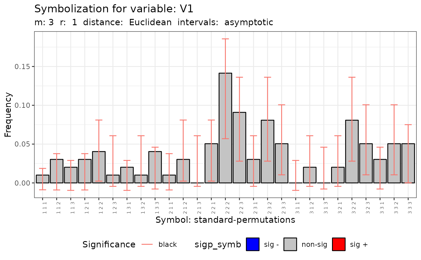 #>
#> [[2]]
#>
#> [[2]]
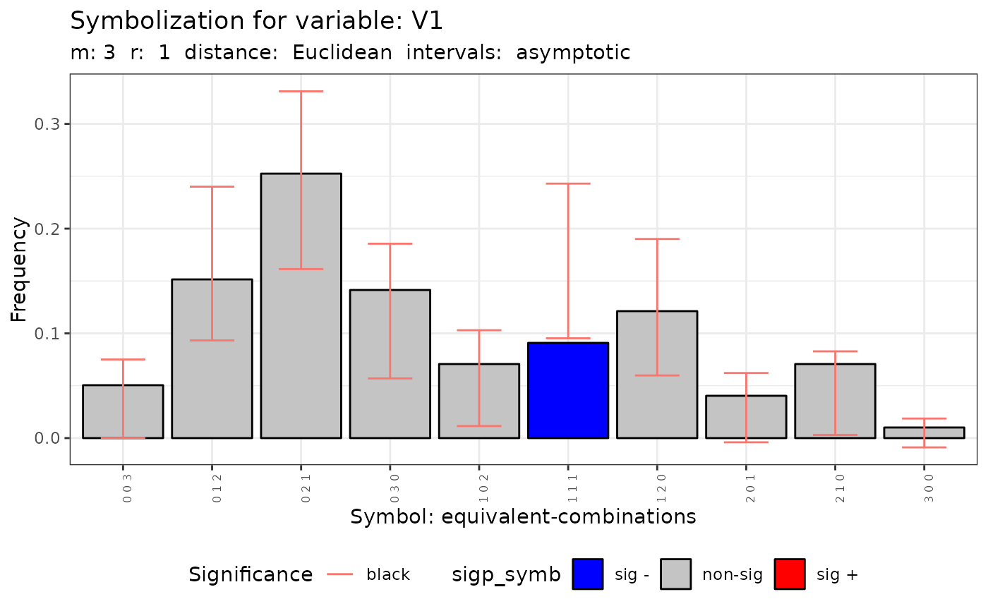 #>
print(q.test)
#> [[1]]
#>
#> Qp (asymptotic distrib.) for standard symbolization based on
#> permutations
#>
#> data: Variable V1 m = 3 r = 1
#> Qp = 17.552, df = 26, p-value = 0.8914
#>
#>
#> [[2]]
#>
#> Qc (asymptotic distrib.) for equivalent symbolization based on
#> combinations
#>
#> data: Variable V1 m = 3 r = 1
#> Qc = 10.054, df = 9, p-value = 0.3461
#>
#>
#> attr(,"class")
#> [1] "spqtest" "list"
# \donttest{
q.test.mc <- Q.test(fx = fx, coor = coor, m = 3, distr = "mc", control = list(nsim = 999))
summary(q.test.mc)
#>
print(q.test)
#> [[1]]
#>
#> Qp (asymptotic distrib.) for standard symbolization based on
#> permutations
#>
#> data: Variable V1 m = 3 r = 1
#> Qp = 17.552, df = 26, p-value = 0.8914
#>
#>
#> [[2]]
#>
#> Qc (asymptotic distrib.) for equivalent symbolization based on
#> combinations
#>
#> data: Variable V1 m = 3 r = 1
#> Qc = 10.054, df = 9, p-value = 0.3461
#>
#>
#> attr(,"class")
#> [1] "spqtest" "list"
# \donttest{
q.test.mc <- Q.test(fx = fx, coor = coor, m = 3, distr = "mc", control = list(nsim = 999))
summary(q.test.mc)
Qualitative Dependence Test (Q)
Distribution: mc. Distance: Euclidean
Q
p.value
k
N
m
R
n
R/n
5k^m
V1 - standard-permutations
V1 - equivalent-combinations
plot(q.test.mc)
#> [[1]]
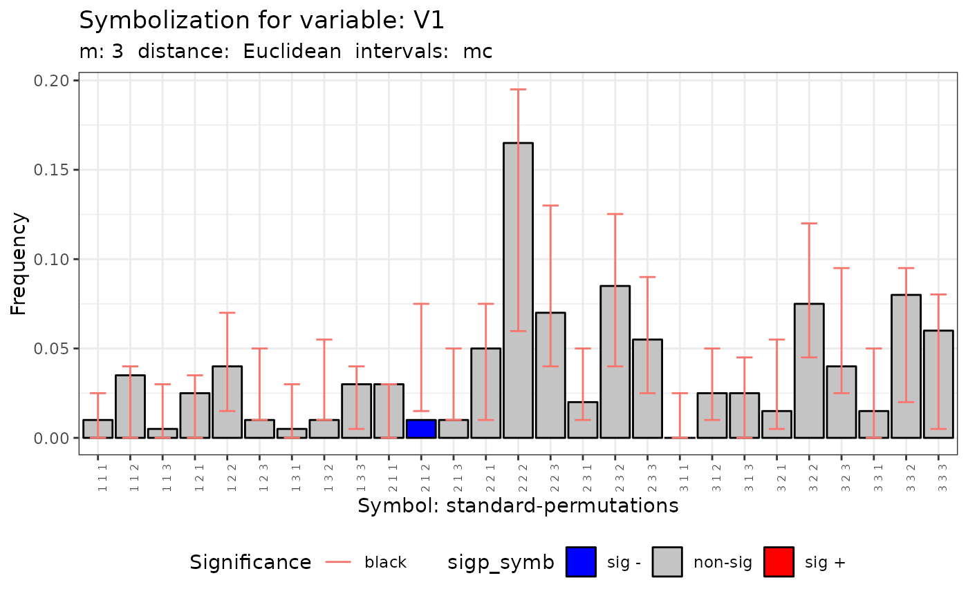 #>
#> [[2]]
#>
#> [[2]]
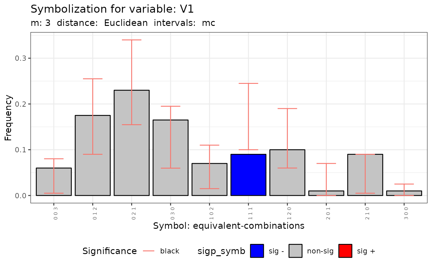 #>
print(q.test.mc)
#> [[1]]
#>
#> Qp (mc distrib.) for symbolization based on permutations
#>
#> data: Variable V1 m = 3 r = 2
#> Qp = 61.649, df = NA, p-value = 0.002
#>
#>
#> [[2]]
#>
#> Qc (mc distrib.) for symbolization based on combinations
#>
#> data: Variable V1 m = 3 r = 2
#> Qc = 35.472, df = NA, p-value = 0.01
#>
#>
#> attr(,"class")
#> [1] "spqtest" "list"
# Case 2: With a sf object
data("FastFood.sf")
f1 <- ~ Type
q.test <- Q.test(formula = f1, data = FastFood.sf, m = c(3, 4),
r = c(1, 2, 3), control = list(distance ="Euclidean"))
summary(q.test)
#>
print(q.test.mc)
#> [[1]]
#>
#> Qp (mc distrib.) for symbolization based on permutations
#>
#> data: Variable V1 m = 3 r = 2
#> Qp = 61.649, df = NA, p-value = 0.002
#>
#>
#> [[2]]
#>
#> Qc (mc distrib.) for symbolization based on combinations
#>
#> data: Variable V1 m = 3 r = 2
#> Qc = 35.472, df = NA, p-value = 0.01
#>
#>
#> attr(,"class")
#> [1] "spqtest" "list"
# Case 2: With a sf object
data("FastFood.sf")
f1 <- ~ Type
q.test <- Q.test(formula = f1, data = FastFood.sf, m = c(3, 4),
r = c(1, 2, 3), control = list(distance ="Euclidean"))
summary(q.test)
Qualitative Dependence Test (Q)
Distribution: asymptotic. Distance: Euclidean
Q
df
p.value
k
N
m
r
R
n
R/n
5k^m
Type - standard-permutations
Type - equivalent-combinations
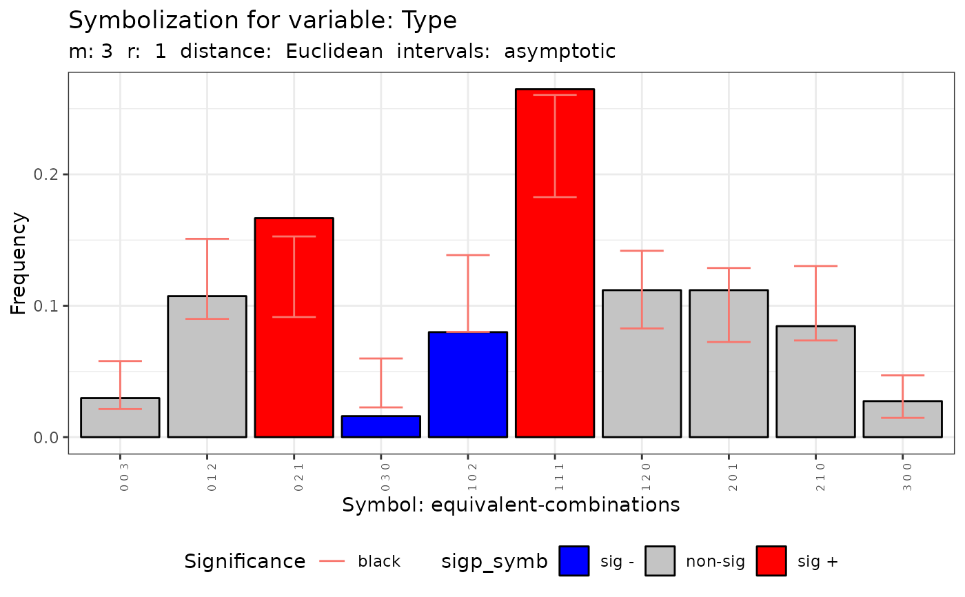
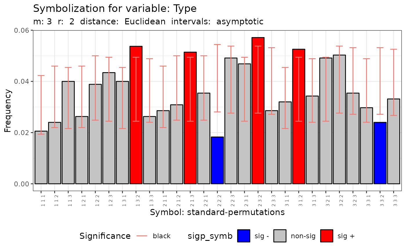
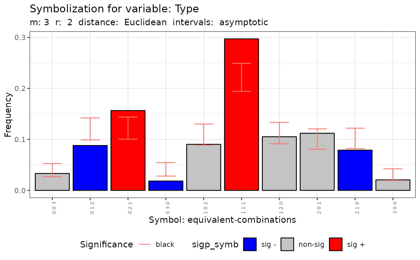
plot(q.test)
#> [[1]]
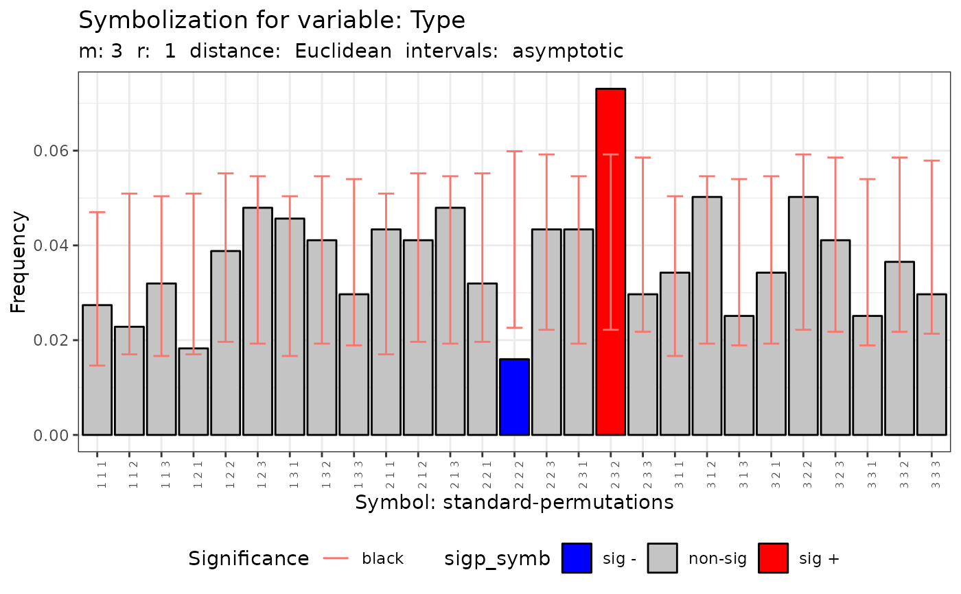 #>
#> [[2]]
#>
#> [[2]]
 #>
#> [[3]]
#>
#> [[3]]
 #>
#> [[4]]
#>
#> [[4]]
 #>
#> [[5]]
#>
#> [[5]]
 #>
#> [[6]]
#>
#> [[6]]
 #>
#> [[7]]
#>
#> [[7]]
 #>
#> [[8]]
#>
#> [[8]]
 #>
#> [[9]]
#>
#> [[9]]
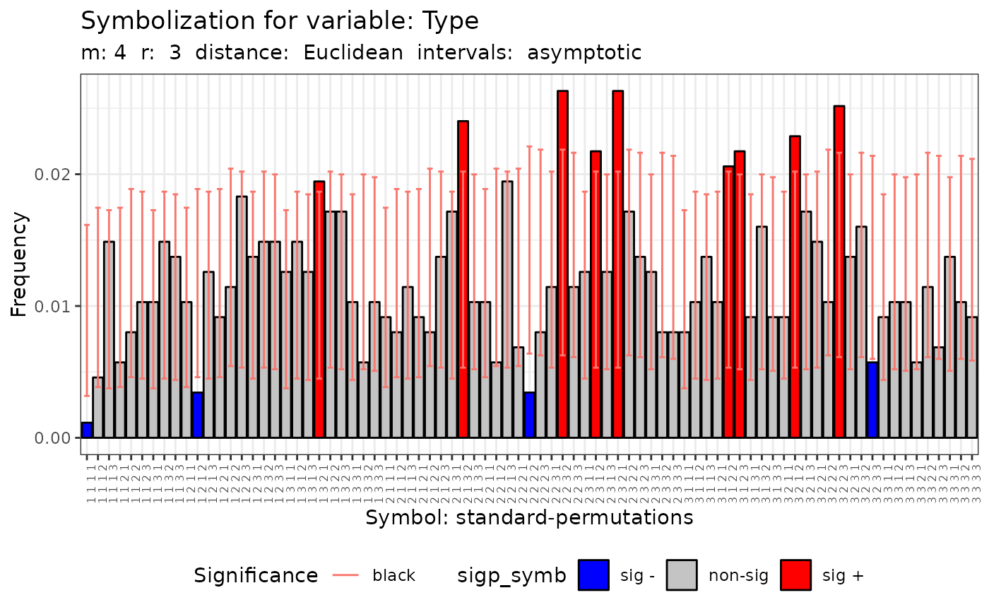 #>
#> [[10]]
#>
#> [[10]]
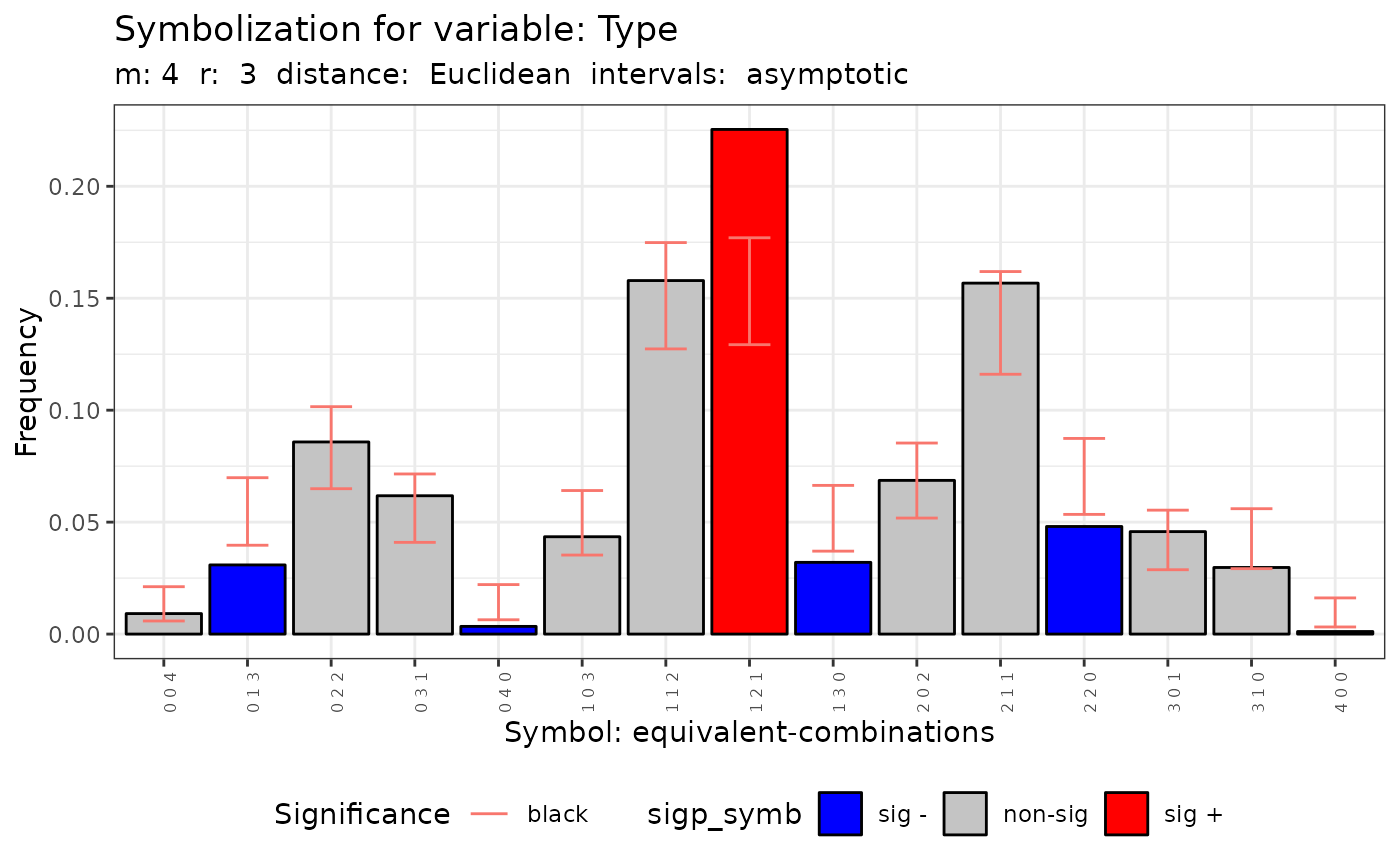 #>
print(q.test)
#> [[1]]
#>
#> Qp (asymptotic distrib.) for standard symbolization based on
#> permutations
#>
#> data: Variable Type m = 3 r = 1
#> Qp = 40.102, df = 26, p-value = 0.03812
#>
#>
#> [[2]]
#>
#> Qc (asymptotic distrib.) for equivalent symbolization based on
#> combinations
#>
#> data: Variable Type m = 3 r = 1
#> Qc = 26.507, df = 9, p-value = 0.001687
#>
#>
#> [[3]]
#>
#> Qp (asymptotic distrib.) for standard symbolization based on
#> permutations
#>
#> data: Variable Type m = 3 r = 2
#> Qp = 71.712, df = 26, p-value = 3.725e-06
#>
#>
#> [[4]]
#>
#> Qc (asymptotic distrib.) for equivalent symbolization based on
#> combinations
#>
#> data: Variable Type m = 3 r = 2
#> Qc = 64.671, df = 9, p-value = 1.672e-10
#>
#>
#> [[5]]
#>
#> Qp (asymptotic distrib.) for standard symbolization based on
#> permutations
#>
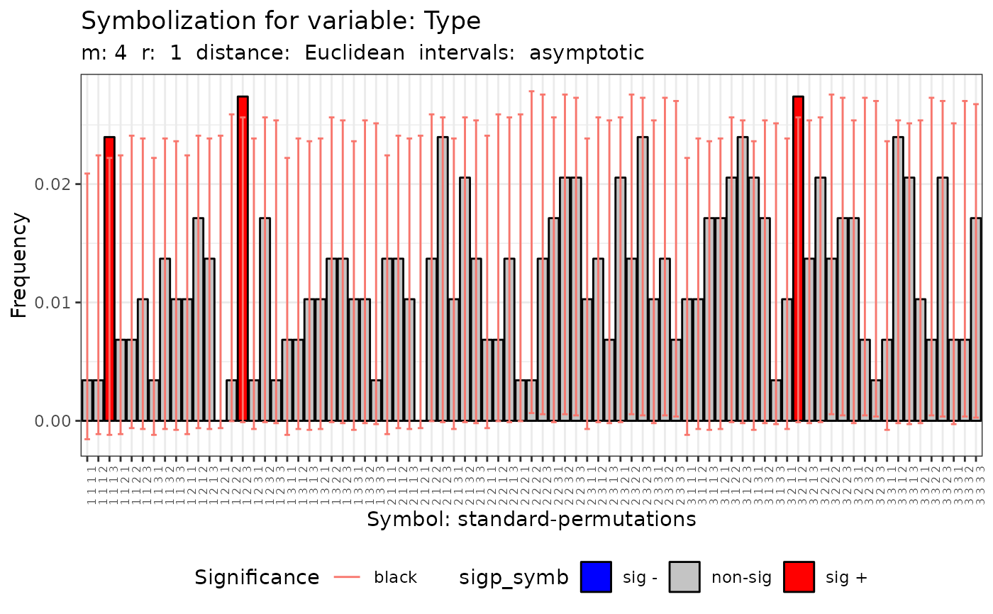
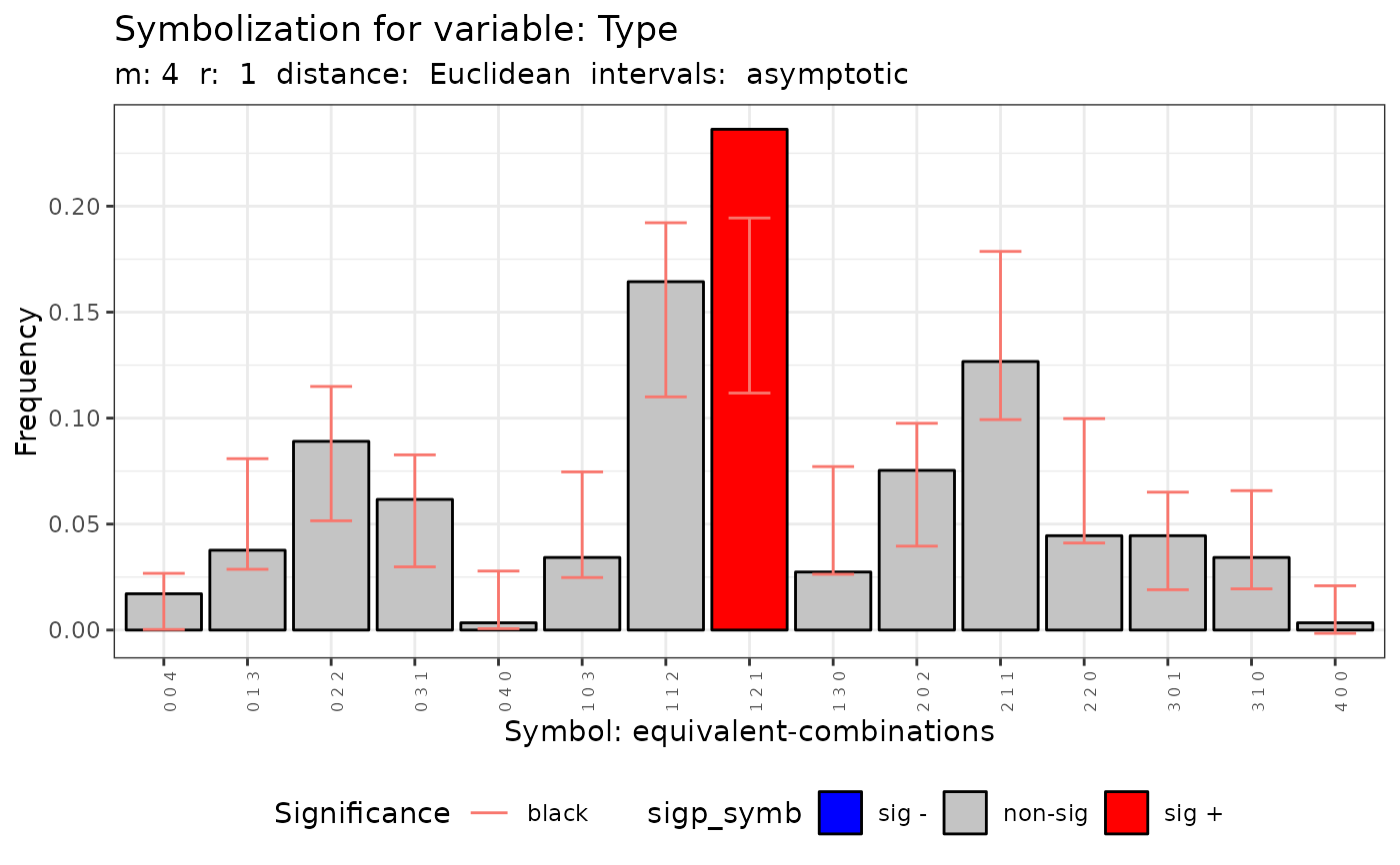
#> data: Variable Type m = 4 r = 1
#> Qp = 89.017, df = 80, p-value = 0.2297
#>
#>
#> [[6]]
#>
#> Qc (asymptotic distrib.) for equivalent symbolization based on
#> combinations
#>
#> data: Variable Type m = 4 r = 1
#> Qc = 28.831, df = 14, p-value = 0.01102
#>
#>
#> [[7]]
#>
#> Qp (asymptotic distrib.) for standard symbolization based on
#> permutations
#>
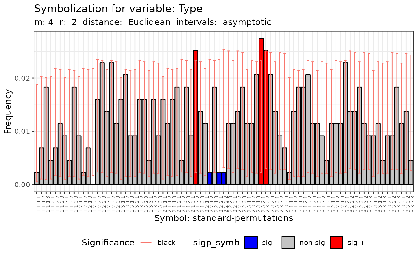
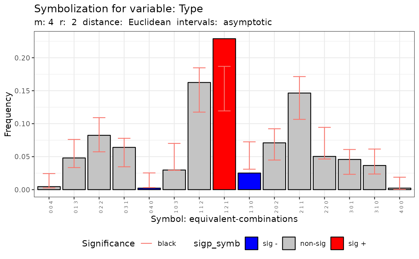
#> data: Variable Type m = 4 r = 2
#> Qp = 115.69, df = 80, p-value = 0.005592
#>
#>
#> [[8]]
#>
#> Qc (asymptotic distrib.) for equivalent symbolization based on
#> combinations
#>
#> data: Variable Type m = 4 r = 2
#> Qc = 44.19, df = 14, p-value = 5.516e-05
#>
#>
#> [[9]]
#>
#> Qp (asymptotic distrib.) for standard symbolization based on
#> permutations
#>
#> data: Variable Type m = 4 r = 3
#> Qp = 151.65, df = 80, p-value = 2.375e-06
#>
#>
#> [[10]]
#>
#> Qc (asymptotic distrib.) for equivalent symbolization based on
#> combinations
#>
#> data: Variable Type m = 4 r = 3
#> Qc = 81.256, df = 14, p-value = 1.654e-11
#>
#>
#> attr(,"class")
#> [1] "spqtest" "list"
# Case 3: With a sf object with isolated areas
data("provinces_spain")
sf::sf_use_s2(FALSE)
#> Spherical geometry (s2) switched off
provinces_spain$Mal2Fml<- factor(provinces_spain$Mal2Fml > 100)
levels(provinces_spain$Mal2Fml) = c("men","woman")
provinces_spain$Older <- cut(provinces_spain$Older, breaks = c(-Inf,19,22.5,Inf))
levels(provinces_spain$Older) = c("low","middle","high")
f1 <- ~ Older + Mal2Fml
q.test <- Q.test(formula = f1,
data = provinces_spain, m = 3, r = 1, control = list(seedinit = 1111))
summary(q.test)
#>
print(q.test)
#> [[1]]
#>
#> Qp (asymptotic distrib.) for standard symbolization based on
#> permutations
#>
#> data: Variable Type m = 3 r = 1
#> Qp = 40.102, df = 26, p-value = 0.03812
#>
#>
#> [[2]]
#>
#> Qc (asymptotic distrib.) for equivalent symbolization based on
#> combinations
#>
#> data: Variable Type m = 3 r = 1
#> Qc = 26.507, df = 9, p-value = 0.001687
#>
#>
#> [[3]]
#>
#> Qp (asymptotic distrib.) for standard symbolization based on
#> permutations
#>
#> data: Variable Type m = 3 r = 2
#> Qp = 71.712, df = 26, p-value = 3.725e-06
#>
#>
#> [[4]]
#>
#> Qc (asymptotic distrib.) for equivalent symbolization based on
#> combinations
#>
#> data: Variable Type m = 3 r = 2
#> Qc = 64.671, df = 9, p-value = 1.672e-10
#>
#>
#> [[5]]
#>
#> Qp (asymptotic distrib.) for standard symbolization based on
#> permutations
#>
#> data: Variable Type m = 4 r = 1
#> Qp = 89.017, df = 80, p-value = 0.2297
#>
#>
#> [[6]]
#>
#> Qc (asymptotic distrib.) for equivalent symbolization based on
#> combinations
#>
#> data: Variable Type m = 4 r = 1
#> Qc = 28.831, df = 14, p-value = 0.01102
#>
#>
#> [[7]]
#>
#> Qp (asymptotic distrib.) for standard symbolization based on
#> permutations
#>
#> data: Variable Type m = 4 r = 2
#> Qp = 115.69, df = 80, p-value = 0.005592
#>
#>
#> [[8]]
#>
#> Qc (asymptotic distrib.) for equivalent symbolization based on
#> combinations
#>
#> data: Variable Type m = 4 r = 2
#> Qc = 44.19, df = 14, p-value = 5.516e-05
#>
#>
#> [[9]]
#>
#> Qp (asymptotic distrib.) for standard symbolization based on
#> permutations
#>
#> data: Variable Type m = 4 r = 3
#> Qp = 151.65, df = 80, p-value = 2.375e-06
#>
#>
#> [[10]]
#>
#> Qc (asymptotic distrib.) for equivalent symbolization based on
#> combinations
#>
#> data: Variable Type m = 4 r = 3
#> Qc = 81.256, df = 14, p-value = 1.654e-11
#>
#>
#> attr(,"class")
#> [1] "spqtest" "list"
# Case 3: With a sf object with isolated areas
data("provinces_spain")
sf::sf_use_s2(FALSE)
#> Spherical geometry (s2) switched off
provinces_spain$Mal2Fml<- factor(provinces_spain$Mal2Fml > 100)
levels(provinces_spain$Mal2Fml) = c("men","woman")
provinces_spain$Older <- cut(provinces_spain$Older, breaks = c(-Inf,19,22.5,Inf))
levels(provinces_spain$Older) = c("low","middle","high")
f1 <- ~ Older + Mal2Fml
q.test <- Q.test(formula = f1,
data = provinces_spain, m = 3, r = 1, control = list(seedinit = 1111))
summary(q.test)
Qualitative Dependence Test (Q)
Distribution: asymptotic. Distance: Euclidean
Q
df
p.value
k
N
m
r
R
n
R/n
5k^m
Older - standard-permutations
Older - equivalent-combinations
Mal2Fml - standard-permutations
Mal2Fml - equivalent-combinations
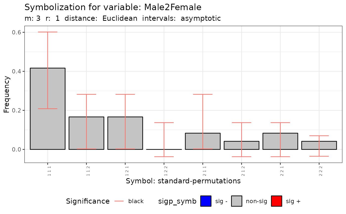
print(q.test)
#> [[1]]
#>
#> Qp (asymptotic distrib.) for standard symbolization based on
#> permutations
#>
#> data: Variable Older m = 3 r = 1
#> Qp = 29.4, df = 26, p-value = 0.2932
#>
#>
#> [[2]]
#>
#> Qc (asymptotic distrib.) for equivalent symbolization based on
#> combinations
#>
#> data: Variable Older m = 3 r = 1
#> Qc = 8.9526, df = 9, p-value = 0.4417
#>
#>
#> [[3]]
#>
#> Qp (asymptotic distrib.) for standard symbolization based on
#> permutations
#>
#> data: Variable Mal2Fml m = 3 r = 1
#> Qp = 4.3369, df = 7, p-value = 0.7403
#>
#>
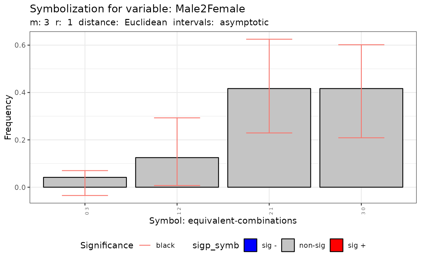
#> [[4]]
#>
#> Qc (asymptotic distrib.) for equivalent symbolization based on
#> combinations
#>
#> data: Variable Mal2Fml m = 3 r = 1
#> Qc = 0.69051, df = 3, p-value = 0.8754
#>
#>
#> attr(,"class")
#> [1] "spqtest" "list"
plot(q.test)
#> [[1]]
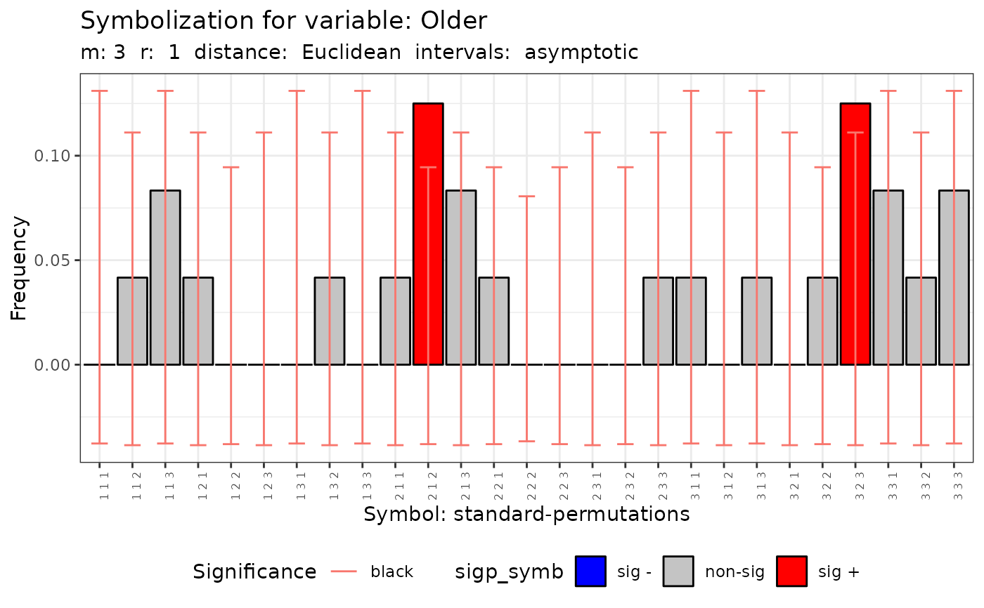 #>
#> [[2]]
#>
#> [[2]]
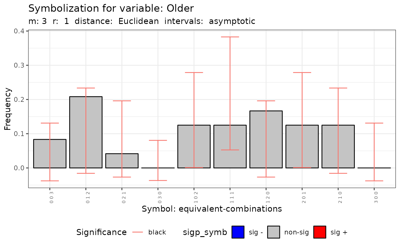 #>
#> [[3]]
#>
#> [[3]]
 #>
#> [[4]]
#>
#> [[4]]
 #>
q.test.mc <- Q.test(formula = f1, data = provinces_spain, m = 4, r = 3, distr = "mc",
control = list(seedinit = 1111))
summary(q.test.mc)
Qualitative Dependence Test (Q)
Distribution: mc. Distance: Euclidean
Q
p.value
k
N
m
R
n
R/n
5k^m
Older - standard-permutations
Older - equivalent-combinations
Mal2Fml - standard-permutations
Mal2Fml - equivalent-combinations
print(q.test.mc)
#> [[1]]
#>
#> Qp (mc distrib.) for symbolization based on permutations
#>
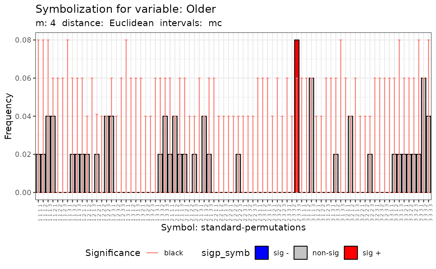
#> data: Variable Older m = 4 r = 3
#> Qp = 92.278, df = NA, p-value = 0.262
#>
#>
#> [[2]]
#>
#> Qc (mc distrib.) for symbolization based on combinations
#>
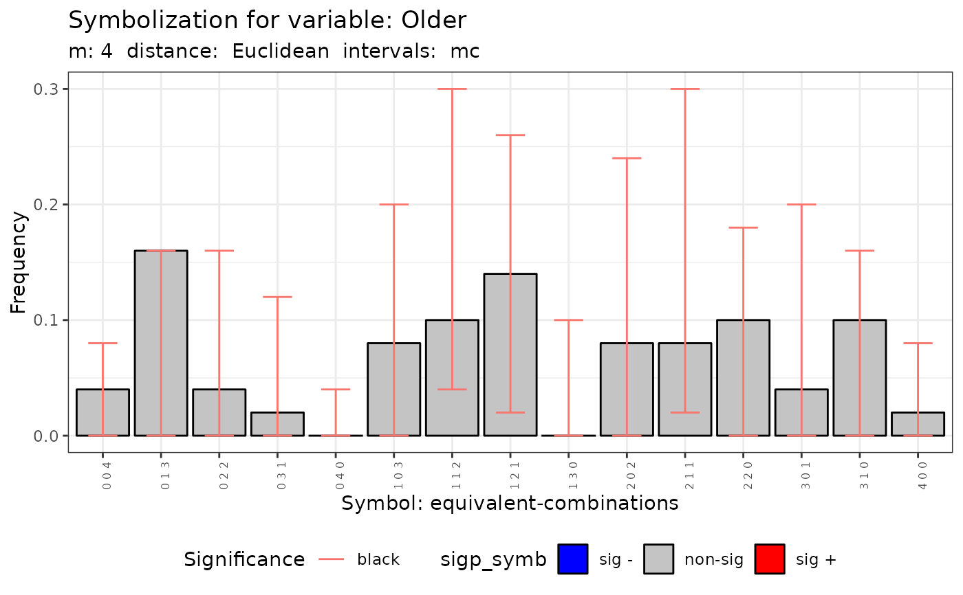
#> data: Variable Older m = 4 r = 3
#> Qc = 20.096, df = NA, p-value = 0.468
#>
#>
#> [[3]]
#>
#> Qp (mc distrib.) for symbolization based on permutations
#>
#> data: Variable Mal2Fml m = 4 r = 3
#> Qp = 18.062, df = NA, p-value = 0.458
#>
#>
#> [[4]]
#>
#> Qc (mc distrib.) for symbolization based on combinations
#>
#> data: Variable Mal2Fml m = 4 r = 3
#> Qc = 6.3535, df = NA, p-value = 0.313
#>
#>
#> attr(,"class")
#> [1] "spqtest" "list"
plot(q.test.mc)
#> [[1]]
 #>
#> [[2]]
#>
#> [[2]]
 #>
#> [[3]]
#>
#> [[3]]
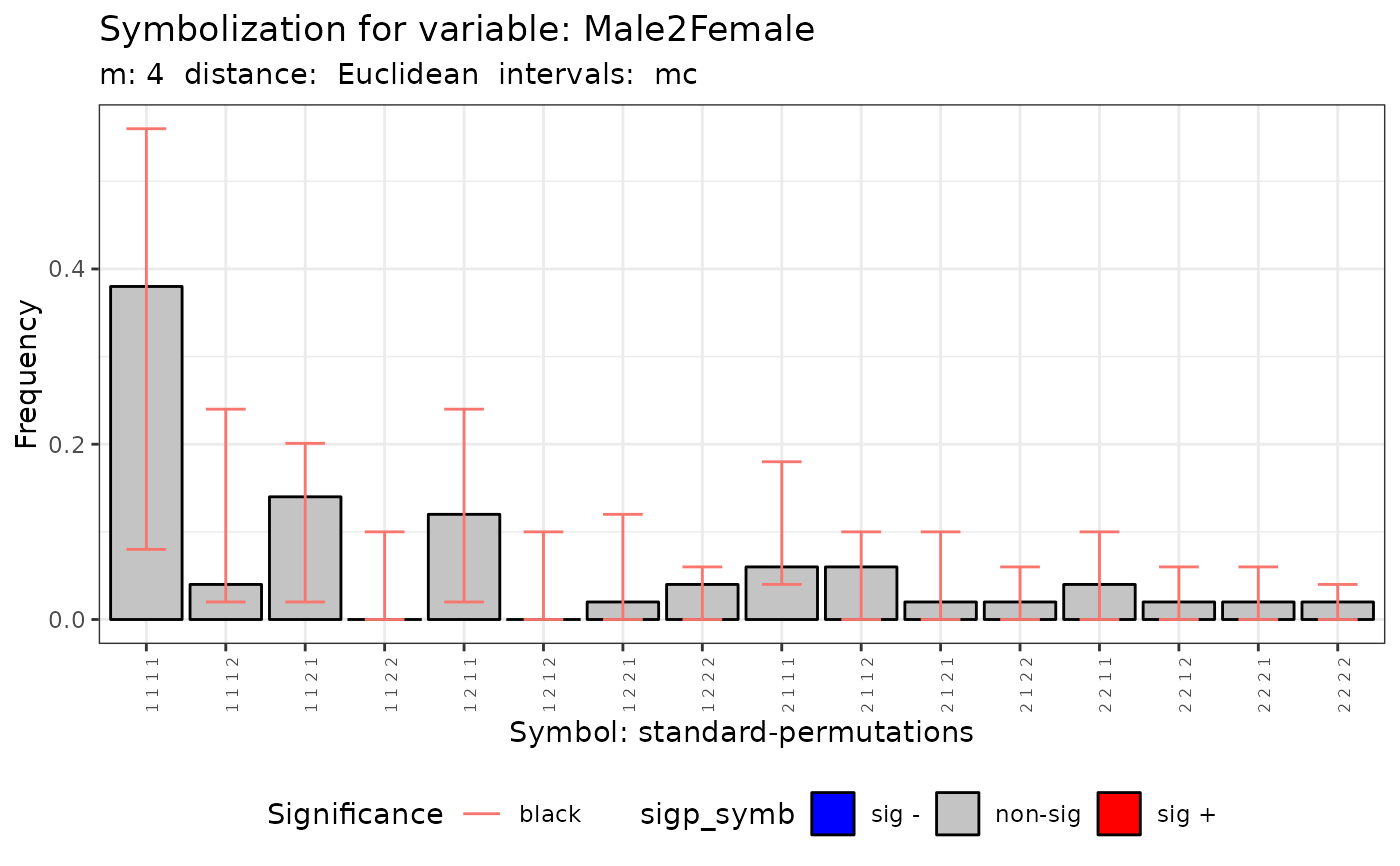 #>
#> [[4]]
#>
#> [[4]]
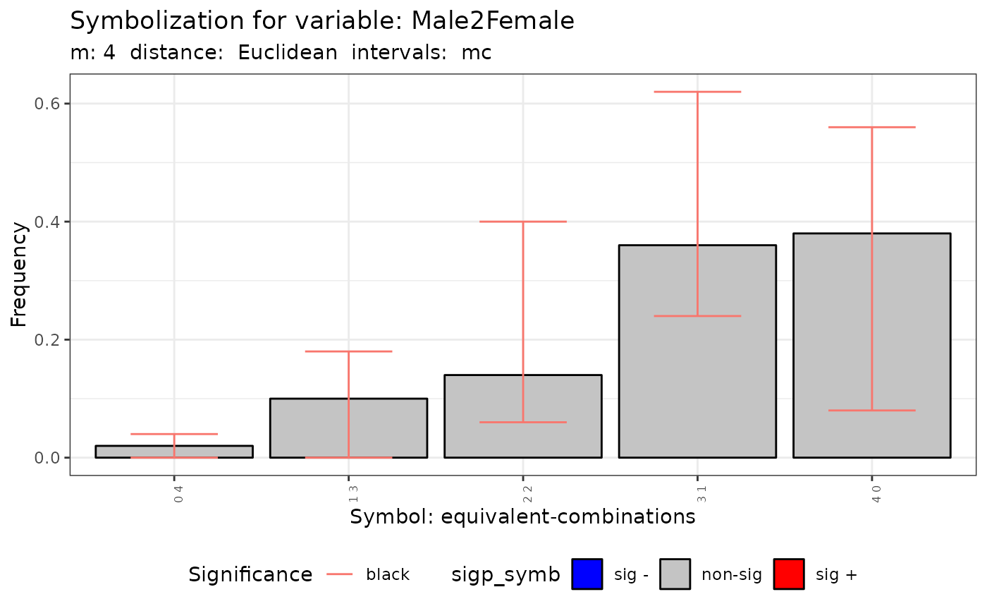 #>
# Case 4: Examples with multipolygons
library(sf)
#> Linking to GEOS 3.12.1, GDAL 3.8.4, PROJ 9.4.0; sf_use_s2() is FALSE
fname <- system.file("shape/nc.shp", package="sf")
nc <- sf::st_read(fname)
#> Reading layer `nc' from data source
#> `/home/runner/work/_temp/Library/sf/shape/nc.shp' using driver `ESRI Shapefile'
#> Simple feature collection with 100 features and 14 fields
#> Geometry type: MULTIPOLYGON
#> Dimension: XY
#> Bounding box: xmin: -84.32385 ymin: 33.88199 xmax: -75.45698 ymax: 36.58965
#> Geodetic CRS: NAD27
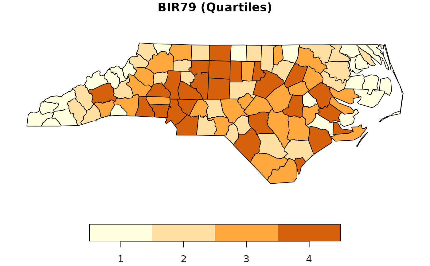
qb79 <- quantile(nc$BIR79)
nc$QBIR79 <- (nc$BIR79 > qb79[2]) + (nc$BIR79 > qb79[3]) +
(nc$BIR79 >= qb79[4]) + 1
nc$QBIR79 <- as.factor(nc$QBIR79)
plot(nc["QBIR79"], pal = c("#FFFEDE","#FFDFA2", "#FFA93F", "#D5610D"),
main = "BIR79 (Quartiles)")
#>
# Case 4: Examples with multipolygons
library(sf)
#> Linking to GEOS 3.12.1, GDAL 3.8.4, PROJ 9.4.0; sf_use_s2() is FALSE
fname <- system.file("shape/nc.shp", package="sf")
nc <- sf::st_read(fname)
#> Reading layer `nc' from data source
#> `/home/runner/work/_temp/Library/sf/shape/nc.shp' using driver `ESRI Shapefile'
#> Simple feature collection with 100 features and 14 fields
#> Geometry type: MULTIPOLYGON
#> Dimension: XY
#> Bounding box: xmin: -84.32385 ymin: 33.88199 xmax: -75.45698 ymax: 36.58965
#> Geodetic CRS: NAD27
qb79 <- quantile(nc$BIR79)
nc$QBIR79 <- (nc$BIR79 > qb79[2]) + (nc$BIR79 > qb79[3]) +
(nc$BIR79 >= qb79[4]) + 1
nc$QBIR79 <- as.factor(nc$QBIR79)
plot(nc["QBIR79"], pal = c("#FFFEDE","#FFDFA2", "#FFA93F", "#D5610D"),
main = "BIR79 (Quartiles)")
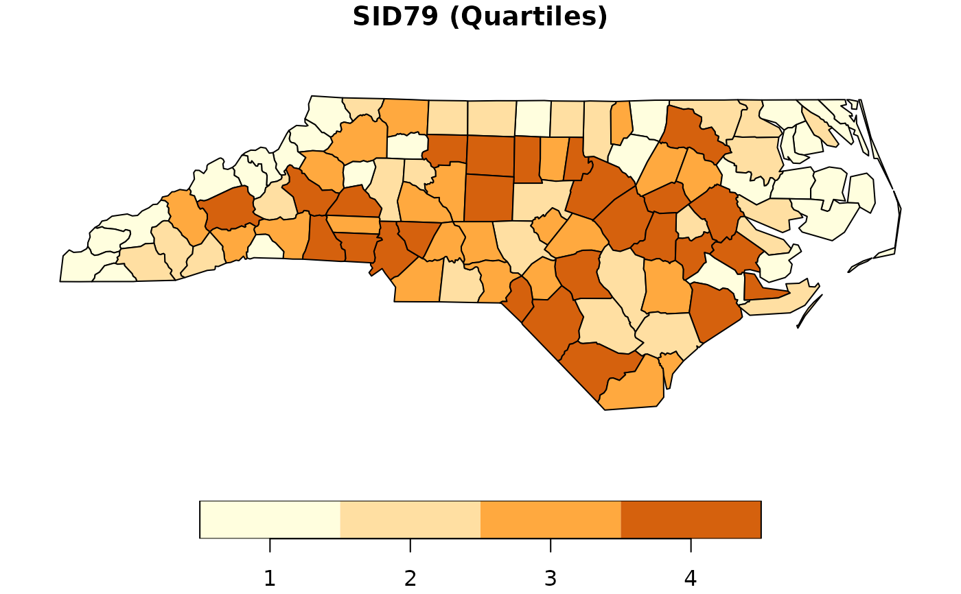
 sid79 <- quantile(nc$SID79)
nc$QSID79 <- (nc$SID79 > sid79[2]) + (nc$SID79 > sid79[3]) +
(nc$SID79 >= sid79[4]) + 1
nc$QSID79 <- as.factor(nc$QSID79)
plot(nc["QSID79"], pal = c("#FFFEDE","#FFDFA2", "#FFA93F", "#D5610D"),
main = "SID79 (Quartiles)")
 f1 <- ~ QSID79 + QBIR79
lq1nc <- Q.test(formula = f1, data = nc, m = 5, r = 2,
control = list(seedinit = 1111, dtmaxpc = 0.5, distance = "Euclidean") )
#>
#> Threshold distance: 4.136024
#> None m-surrounding excluded for exceeding
#> the threshold distance
#>
#> Threshold distance: 4.136024
#> None m-surrounding excluded for exceeding
#> the threshold distance
print(lq1nc)
#> [[1]]
#>
#> Qp (asymptotic distrib.) for standard symbolization based on
#> permutations
#>
#> data: Variable QSID79 m = 5 r = 2
#> Qp = 225.84, df = 1023, p-value = 1
#>
#>
#> [[2]]
#>
#> Qc (asymptotic distrib.) for equivalent symbolization based on
#> combinations
#>
#> data: Variable QSID79 m = 5 r = 2
#> Qc = 61.371, df = 55, p-value = 0.2583
#>
#>
#> [[3]]
#>
#> Qp (asymptotic distrib.) for standard symbolization based on
#> permutations
#>
#> data: Variable QBIR79 m = 5 r = 2
#> Qp = 221.81, df = 1023, p-value = 1
#>
#>
#> [[4]]
#>
#> Qc (asymptotic distrib.) for equivalent symbolization based on
#> combinations
#>
#> data: Variable QBIR79 m = 5 r = 2
#> Qc = 59.272, df = 55, p-value = 0.3226
#>
#>
#> attr(,"class")
#> [1] "spqtest" "list"
lq2nc <- Q.test(formula = f1, data = nc, m = 5, r = 2,
control = list(dtmaxpc = 0.2) )
#>
#> Threshold distance: 1.65441
#> Number of m-surroundings excluded for exceeding
#> the threshold distance: 3
#>
#> Index of spatial observations excluded: 19 3 28
#>
#> Threshold distance: 1.65441
#> Number of m-surroundings excluded for exceeding
#> the threshold distance: 3
#>
#> Index of spatial observations excluded: 19 3 28
print(lq2nc)
#> [[1]]
#>
#> Qp (asymptotic distrib.) for standard symbolization based on
#> permutations
#>
#> data: Variable QSID79 m = 5 r = 2
#> Qp = 210.14, df = 1023, p-value = 1
#>
#>
#> [[2]]
#>
#> Qc (asymptotic distrib.) for equivalent symbolization based on
#> combinations
#>
#> data: Variable QSID79 m = 5 r = 2
#> Qc = 62.831, df = 55, p-value = 0.2186
#>
#>
#> [[3]]
#>
#> Qp (asymptotic distrib.) for standard symbolization based on
#> permutations
#>
#> data: Variable QBIR79 m = 5 r = 2
#> Qp = 206.72, df = 1023, p-value = 1
#>
#>
#> [[4]]
#>
#> Qc (asymptotic distrib.) for equivalent symbolization based on
#> combinations
#>
#> data: Variable QBIR79 m = 5 r = 2
#> Qc = 60.539, df = 55, p-value = 0.2828
#>
#>
#> attr(,"class")
#> [1] "spqtest" "list"
lq3nc <- Q.test(formula = f1, data = nc, m = 5, r = 2,
control = list(dtmaxknn = 5) )
print(lq3nc)
#> [[1]]
#>
#> Qp (asymptotic distrib.) for standard symbolization based on
#> permutations
#>
#> data: Variable QSID79 m = 5 r = 2
#> Qp = 43.935, df = 1023, p-value = 1
#>
#>
#> [[2]]
#>
#> Qc (asymptotic distrib.) for equivalent symbolization based on
#> combinations
#>
#> data: Variable QSID79 m = 5 r = 2
#> Qc = 18.923, df = 55, p-value = 1
#>
#>
#> [[3]]
#>
#> Qp (asymptotic distrib.) for standard symbolization based on
#> permutations
#>
#> data: Variable QBIR79 m = 5 r = 2
#> Qp = 44.361, df = 1023, p-value = 1
#>
#>
#> [[4]]
#>
#> Qc (asymptotic distrib.) for equivalent symbolization based on
#> combinations
#>
#> data: Variable QBIR79 m = 5 r = 2
#> Qc = 20.16, df = 55, p-value = 1
#>
#>
#> attr(,"class")
#> [1] "spqtest" "list"
# Case 5: Examples with points and matrix of variables
fx <- matrix(c(nc$QBIR79, nc$QSID79), ncol = 2, byrow = TRUE)
mctr <- suppressWarnings(sf::st_centroid(st_geometry(nc)))
mcoor <- st_coordinates(mctr)[,c("X","Y")]
q.test <- Q.test(fx = fx, coor = mcoor, m = 5, r = 2,
control = list(seedinit = 1111, dtmaxpc = 0.5))
#>
#> Threshold distance: 4.136024
#> None m-surrounding excluded for exceeding
#> the threshold distance
#>
#> Threshold distance: 4.136024
#> None m-surrounding excluded for exceeding
#> the threshold distance
print(q.test)
#> [[1]]
#>
#> Qp (asymptotic distrib.) for standard symbolization based on
#> permutations
#>
#> data: Variable V1 m = 5 r = 2
#> Qp = 221.87, df = 1023, p-value = 1
#>
#>
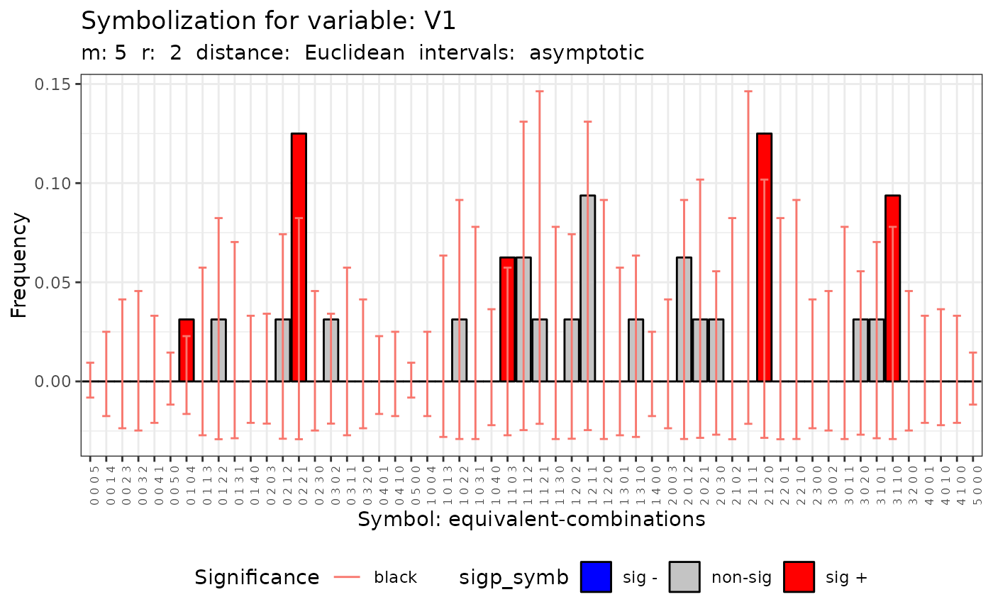
#> [[2]]
#>
#> Qc (asymptotic distrib.) for equivalent symbolization based on
#> combinations
#>
#> data: Variable V1 m = 5 r = 2
#> Qc = 55.411, df = 55, p-value = 0.4591
#>
#>
#> [[3]]
#>
#> Qp (asymptotic distrib.) for standard symbolization based on
#> permutations
#>
#> data: Variable V2 m = 5 r = 2
#> Qp = 220.68, df = 1023, p-value = 1
#>
#>
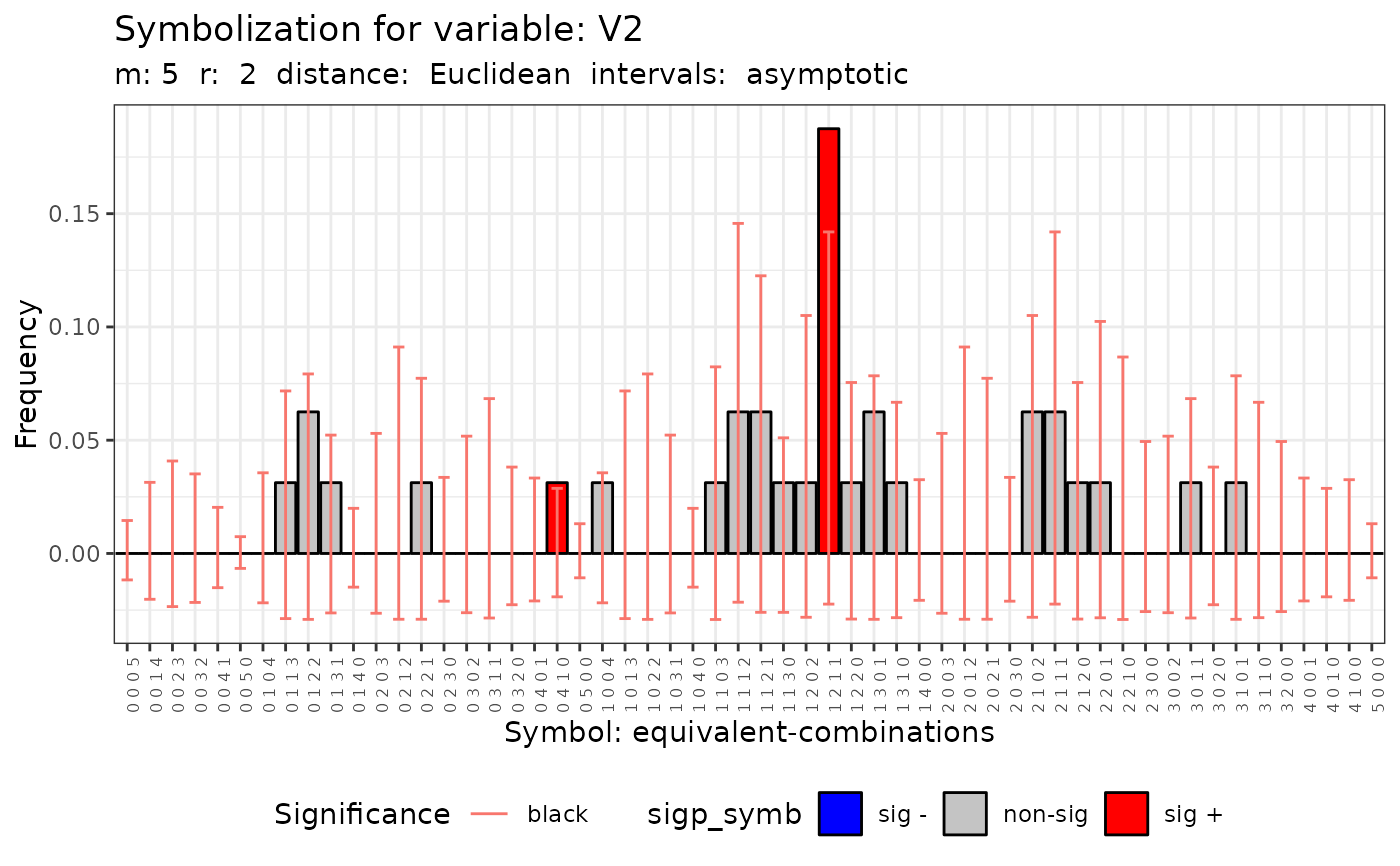
#> [[4]]
#>
#> Qc (asymptotic distrib.) for equivalent symbolization based on
#> combinations
#>
#> data: Variable V2 m = 5 r = 2
#> Qc = 38.975, df = 55, p-value = 0.9498
#>
#>
#> attr(,"class")
#> [1] "spqtest" "list"
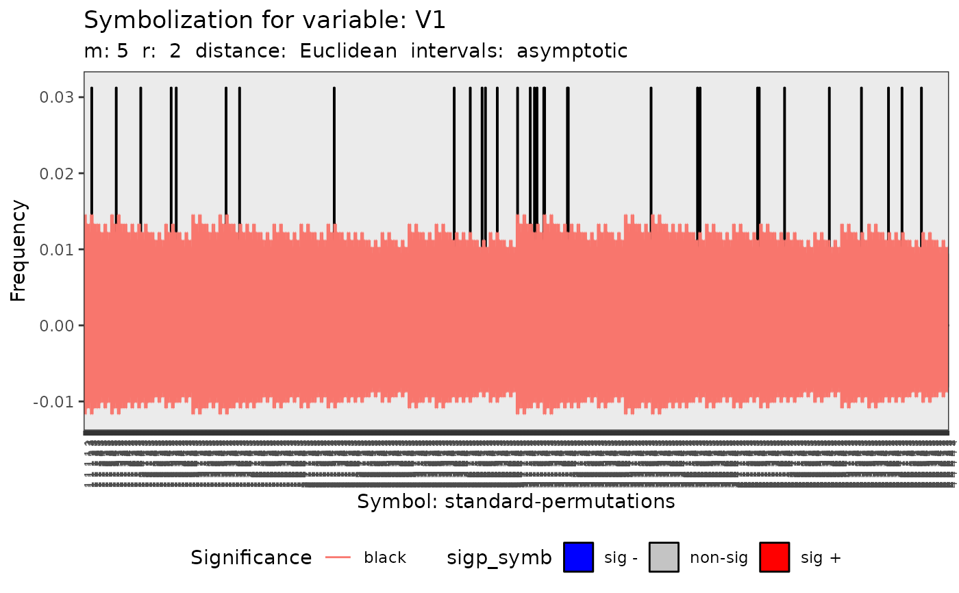
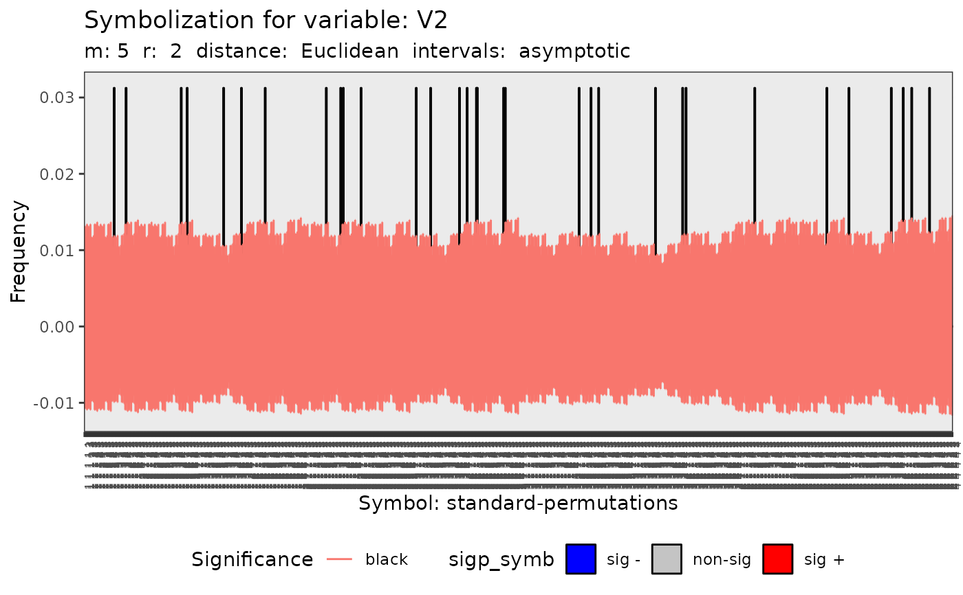
plot(q.test)
#> [[1]]
 #>
#> [[2]]
#>
#> [[2]]
 #>
#> [[3]]
#>
#> [[3]]
 #>
#> [[4]]
#>
#> [[4]]
 #>
# }