This function compute the spatial scan test for Bernoulli and Multinomial categorical spatial process, and detect spatial clusters
Usage
scan.test(formula = NULL, data = NULL, fx = NULL, coor = NULL, case = NULL,
nv = NULL, nsim = NULL, distr = NULL, windows = "circular", listw = NULL,
alternative = "High", minsize = 1, control = list())
Arguments
- formula
a symbolic description of the factor (optional).
- data
an (optional) data frame or a sf object containing the variable to testing for.
- fx
a factor (optional).
- coor
(optional) coordinates of observations.
- case
Only for Bernoulli distribution. A element of factor, there are cases and non-cases for testing for cases versus non-cases
- nv
Maximum windows size, default nv = N/2. The algorithm scan for clusters of geographic size between 1 and the upper limit (nv) defined by the user.
- nsim
Number of permutations.
- distr
distribution of the spatial process: "bernoulli" for two levels or "multinomial" for three or more levels.
- windows
a string to select the type of cluster "circular" (default) of "elliptic".
- listw
only for flexible windows. A neighbours list (an object of the class listw, nb or knn frop spdep) or an adjacency matrix.
- alternative
Only for Bernoulli spatial process. A character string specifying the type of cluster, must be one of "High" (default), "Both" or "Low".
- minsize
Minimum number of observations inside of Most Likely Cluster and secondary clusters.
- control
List of additional control arguments.
Value
A object of the htest and scantest class
method | The type of test applied (). |
fx | Factor included as input to get the scan test. |
MLC | Observations included into the Most Likelihood Cluster (MLC). |
statistic | Value of the scan test (maximum Log-likelihood ratio). |
N | Total number of observations. |
nn | Windows used to get the cluster. |
nv | Maximum number of observations into the cluster. |
data.name | A character string giving the name of the factor. |
coor | coordinates. |
alternative | Only for bernoulli spatial process. A character string describing the alternative hypothesis select by the user. |
p.value | p-value of the scan test. |
cases.expect | Expected cases into the MLC. |
cases.observ | Observed cases into the MLC. |
nsim | Number of permutations. |
scan.mc | a (nsim x 1) vector with the loglik values under bootstrap permutation. |
secondary.clusters | a list with the observations included into the secondary clusters. |
loglik.second | a vector with the value of the secondary scan tests (maximum Log-likelihood ratio). |
p.value.secondary | a vector with the p-value of the secondary scan tests. |
Alternative.MLC | A vector with the observations included in another cluster with the same loglik than MLC. |
Details
Two alternative sets of arguments can be included in this function to compute the scan test:
Option 1: A factor (fx) and coordinates (coor).Option 2: A sf object (data) and the formula to specify the factor. The function consider the coordinates of the centroids of the elements of th sf object.
The spatial scan statistics are widely used in epidemiology, criminology or ecology.
Their purpose is to analyse the spatial distribution of points or geographical
regions by testing the hypothesis of spatial randomness distribution on the
basis of different distributions (e.g. Bernoulli, Poisson or Normal distributions).
The scan.test function obtain the scan statistic for two relevant distributions related
with categorical variables: the Bernoulli and Multinomial distribution.
The spatial scan statistic is based on the likelihood ratio test statistic and
is formulated as follows:
$$\Delta = { \max_{z \in Z,H_A} L(\theta|z) \over \max_{z \in Z,H_0} L(\theta|z)}$$
where Z represents the collection of scanning windows constructed on the study region,
\(H_A\) is an alternative hypothesis, \(H_0\) is a null hypothesis, and \(L(\theta|z)\)
is the likelihood function with parameter \(\theta\) given window Z
.
The null hypothesis says that there is no spatial clustering on the study region, and
the alternative hypothesis is that there is a certain area with high (or low) rates of
outcome variables. The null and alternative hypotheses and the likelihood function may
be expressed in different ways depending on the probability model under consideration.
To test independence in a spatial process, under the null, the type of windows is
irrelevant but under the alternative the elliptic
windows can to identify with more precision the cluster.
For big data sets (N >>) the windows = "elliptic" can be so slowly
Bernoulli version
When we have dichotomous outcome variables, such as cases and noncases of certain
diseases, the Bernoulli model is used. The null hypothesis is written as
$$H_0 : p = q \ \ for \ \ all \ \ Z$$
and the alternative hypothesis is
$$H_A : p \neq q \ \ for \ \ some \ \ Z$$
where p and q are the outcome probabilities (e.g., the probability of being a case)
inside and outside scanning window Z, respectively. Given window Z, the test statistic is:
where cz and nz are the numbers of cases and observations (cases and noncases) within z,
respectively, and C and N are the total numbers of cases and observations in the whole
study region, respectively.
$$\Delta = $$
Multinomial version of the scan test
The multinomial version of the spatial scan statistic is useful to investigate clustering
when a discrete spatial variable can take one and only one of k possible outcomes
that lack intrinsic order information. If the region defined by the moving window
is denoted by Z, the null hypothesis for the statistic can be stated as follows:
$$H_0: p_1 = q_1;p_2 = q_2;...;p_k = q_k$$
where \(p_j\) is the probability of being of event type j inside the window Z,
and \(q_j\) is the probability of being of event type j outside the window.
The alternative hypothesis is that for at least one type event the probability
of being of that type is different inside and outside of the window.
The statistic is built as a likelihood ratio, and takes the following
form after transformation using the natural logarithm:
$$\Delta = \max_Z \{\sum_j \{ S_j^Z log({ S_j^Z \over S^Z }) +
(S_j-S_j^Z) log({ {S_j-S_j^Z} \over {S-S^Z} })\}\}-\sum_j S_j log({ S_j \over S }) $$
where S is the total number of events in the study area and \(S_j\) is the total number
of events of type j. The superscript Z denotes the same but for the sub-region
defined by the moving window.
The theoretical distribution of the statistic under the null hypothesis is not known,
and therefore significance is evaluated numerically by simulating neutral landscapes
(obtained using a random spatial process) and contrasting the empirically calculated
statistic against the frequency of values obtained from the neutral landscapes.
The results of the likelihood ratio serve to identify the most likely cluster,
which is followed by secondary clusters by the expedient of sorting them according to
the magnitude of the test. As usual, significance is assigned by the analyst, and the
cutoff value for significance reflects the confidence of the analyst, or tolerance for error.
When implementing the statistic, the analyst must decide the shape of the
window and the maximum number of cases that any given window can cover.
Currently, analysis can be done using circular or elliptical windows.
Elliptical windows are more time consuming to evaluate but provide greater
flexibility to contrast the distribution of events inside and outside the window,
and are our selected shape in the analyses to follow. Furthermore, it is recommended
that the maximum number of cases entering any given window does not exceed 50\
all available cases.
Control arguments
seedinit | Numerical value for the seed (only for boot version). Default value seedinit=123 |
References
Kulldorff M, Nagarwalla N. (1995). Spatial disease clusters: Detection and Inference. Statistics in Medicine. 14:799-810
Jung I, Kulldorff M, Richard OJ (2010). A spatial scan statistic for multinomial data. Statistics in Medicine. 29(18), 1910-1918
Páez, A., López-Hernández, F.A., Ortega-García, J.A., Ruiz, M. (2016). Clustering and co-occurrence of cancer types: A comparison of techniques with an application to pediatric cancer in Murcia, Spain. Spatial Analysis in Health Geography, 69-90.
Tango T., Takahashi K. (2005). A flexibly shaped spatial scan statistic for detecting clusters, International Journal of Health Geographics 4:11.
Author
| Fernando López | fernando.lopez@upct.es |
| Román Mínguez | roman.minguez@uclm.es |
| Antonio Páez | paezha@gmail.com |
| Manuel Ruiz | manuel.ruiz@upct.es |
Examples
# Case 1: Scan test bernoulli
data(provinces_spain)
sf::sf_use_s2(FALSE)
provinces_spain$Mal2Fml <- factor(provinces_spain$Mal2Fml > 100)
levels(provinces_spain$Mal2Fml) = c("men","woman")
formula <- ~ Mal2Fml
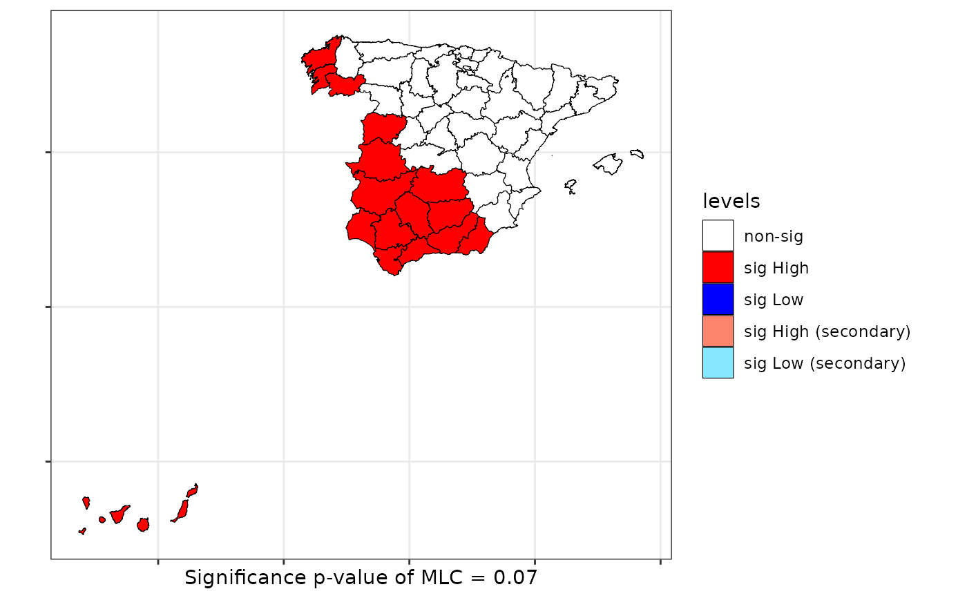
scan <- scan.test(formula = formula, data = provinces_spain, case="men",
nsim = 99, distr = "bernoulli")
print(scan)
#>
#> Scan test. Distribution: bernoulli
#>
#> data: Mal2Fml
#> scan-loglik = 6.0359, p-value = 0.07
#> alternative hypothesis: High
#> sample estimates:
#>
#> Total observations in the MLC = 17.00
#> Expected cases in the MLC = 11.84
#> Observed cases in the MLC = 16.00
#>
summary(scan)
#>
#> Summary of data:
#> Distribution....................: bernoulli
#> Type of cluster (alternative)...: High
#> Number of locations.............: 50
#> Cathegory case..................: men
#> Total number of observations....: 37
#> Names of cathegories............: men woman
#> Total per category..............: 37 13
#> Percent per category............: 0.74 0.26
#> ---------------------------------
#>
#> Scan statistic: Most Likely Cluster
#> Total observations in the MLC........: 17
#> Names of cathegories.................: men woman
#> Percent per category total...........: 0.74 0.26
#> Percent per category inside cluster..: 0.94 0.06
#> Value of statisitic (loglik ratio)...: 6.0359
#> p-value..............................: 0.07
#>
#> IDs of cluster detect:
#> Location IDs included...: 37 34 20 11 40 28 6 14 10 18 35 36 22 31 13 15 4
#> ---------------------------------
#>
#>
#> Secondary Cluster. Number 1
#> Total observations in secondary cluster.: 23
#> Names of cathegories.................: men woman
#> Percent per category total...........: 0.74 0.26
#> Percent per category inside cluster..: 0.61 0.39
#> Value of statisitic (loglik ratio)...: 5.4635
#> p-value..............................: 0.15
#> Location IDs included................: 41 25 19 1 9 30 48 39 50 27 46 16 42 33 38 45 43 5 21 12 2 44 13
#>
#>
#> Secondary Cluster. Number 2
#> Total observations in secondary cluster.: 2
#> Names of cathegories.................: men woman
#> Percent per category total...........: 0.74 0.26
#> Percent per category inside cluster..: 1 0
#> Value of statisitic (loglik ratio)...: 0.3047
#> p-value..............................: 0.99
#> Location IDs included................: 3 44
#>
#>
#> Secondary Cluster. Number 3
#> Total observations in secondary cluster.: 2
#> Names of cathegories.................: men woman
#> Percent per category total...........: 0.74 0.26
#> Percent per category inside cluster..: 0.5 0.5
#> Value of statisitic (loglik ratio)...: 0.3047
#> p-value..............................: 0.99
#> Location IDs included................: 7 8
#>
#>
#> Secondary Cluster. Number 4
#> Total observations in secondary cluster.: 2
#> Names of cathegories.................: men woman
#> Percent per category total...........: 0.74 0.26
#> Percent per category inside cluster..: 1 0
#> Value of statisitic (loglik ratio)...: 0.3047
#> p-value..............................: 0.99
#> Location IDs included................: 17 8
#>
#>
#> Secondary Cluster. Number 5
#> Total observations in secondary cluster.: 2
#> Names of cathegories.................: men woman
#> Percent per category total...........: 0.74 0.26
#> Percent per category inside cluster..: 0.5 0.5
#> Value of statisitic (loglik ratio)...: 0.3047
#> p-value..............................: 0.99
#> Location IDs included................: 24 49
plot(scan, sf = provinces_spain)
 # \donttest{
## With maximum number of neighborhood
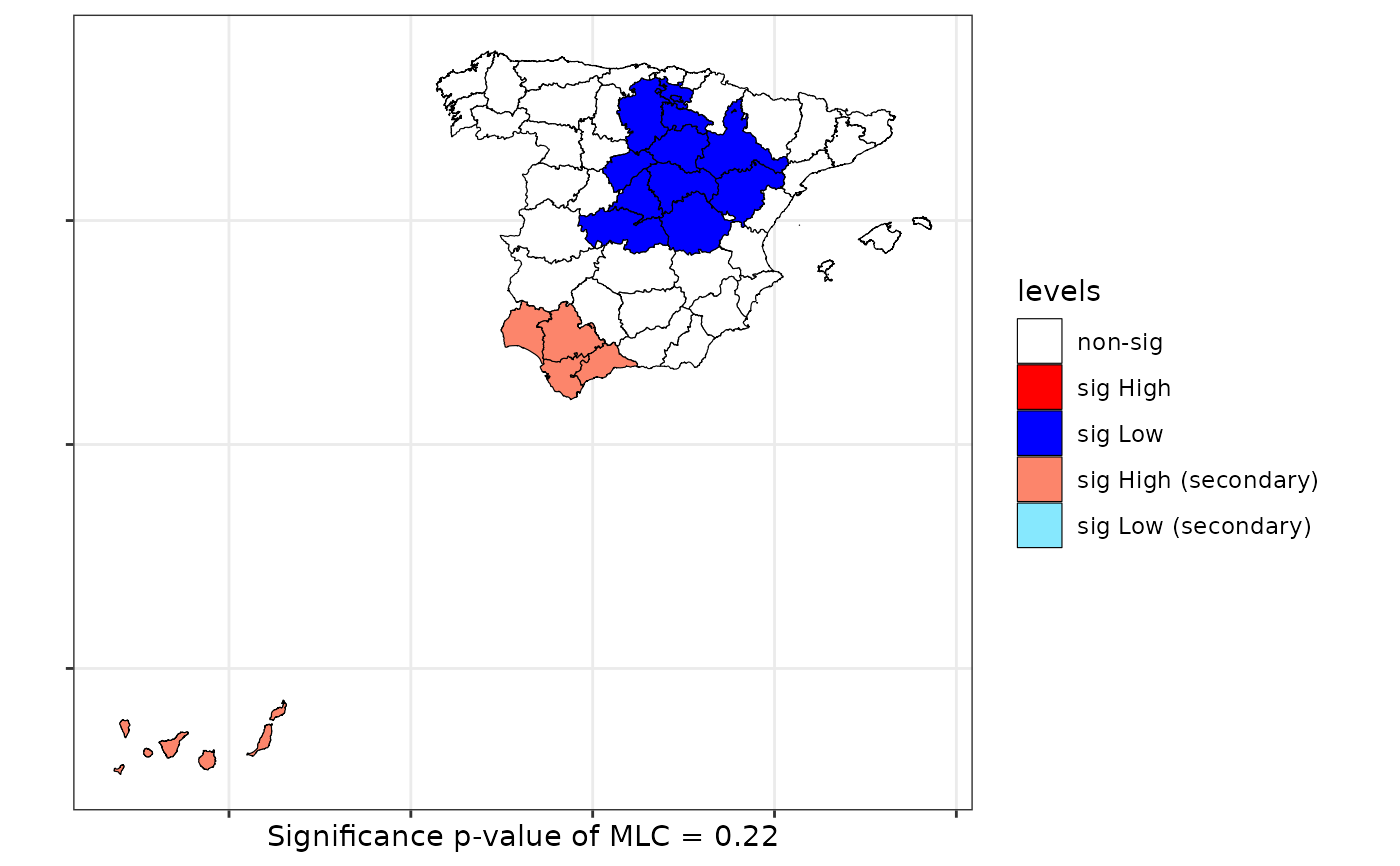
scan <- scan.test(formula = formula, data = provinces_spain, case = "woman",
nsim = 99, distr = "bernoulli")
print(scan)
#>
#> Scan test. Distribution: bernoulli
#>
#> data: Mal2Fml
#> scan-loglik = 5.6358, p-value = 0.22
#> alternative hypothesis: High
#> sample estimates:
#>
#> Total observations in the MLC = 11.00
#> Expected cases in the MLC = 7.02
#> Observed cases in the MLC = 7.00
#>
plot(scan, sf = provinces_spain)
# \donttest{
## With maximum number of neighborhood
scan <- scan.test(formula = formula, data = provinces_spain, case = "woman",
nsim = 99, distr = "bernoulli")
print(scan)
#>
#> Scan test. Distribution: bernoulli
#>
#> data: Mal2Fml
#> scan-loglik = 5.6358, p-value = 0.22
#> alternative hypothesis: High
#> sample estimates:
#>
#> Total observations in the MLC = 11.00
#> Expected cases in the MLC = 7.02
#> Observed cases in the MLC = 7.00
#>
plot(scan, sf = provinces_spain)
 ## With elliptic windows
scan <- scan.test(formula = formula, data = provinces_spain, case = "men", nv = 25,
nsim = 99, distr = "bernoulli", windows ="elliptic")
print(scan)
#>
#> Scan test. Distribution: bernoulli
#>
#> data: Mal2Fml
#> scan-loglik = 7.038, p-value < 2.2e-16
#> alternative hypothesis: High
#> sample estimates:
#>
#> Total observations in the MLC = 19.00
#> Expected cases in the MLC = 62.16
#> Observed cases in the MLC = 18.00
#>
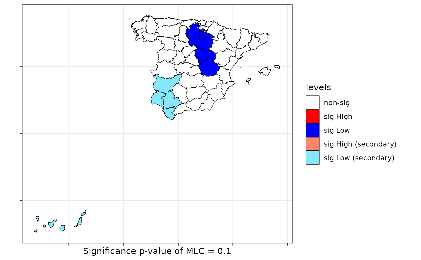
scan <- scan.test(formula = formula, data = provinces_spain, case = "men", nv = 15,
nsim = 99, distr = "bernoulli", windows ="elliptic", alternative = "Low")
print(scan)
#>
#> Scan test. Distribution: bernoulli
#>
#> data: Mal2Fml
#> scan-loglik = 5.9143, p-value = 0.1
#> alternative hypothesis: Low
#> sample estimates:
#>
#> Total observations in the MLC = 5.00
#> Expected cases in the MLC = 51.06
#> Observed cases in the MLC = 1.00
#>
plot(scan, sf = provinces_spain)
## With elliptic windows
scan <- scan.test(formula = formula, data = provinces_spain, case = "men", nv = 25,
nsim = 99, distr = "bernoulli", windows ="elliptic")
print(scan)
#>
#> Scan test. Distribution: bernoulli
#>
#> data: Mal2Fml
#> scan-loglik = 7.038, p-value < 2.2e-16
#> alternative hypothesis: High
#> sample estimates:
#>
#> Total observations in the MLC = 19.00
#> Expected cases in the MLC = 62.16
#> Observed cases in the MLC = 18.00
#>
scan <- scan.test(formula = formula, data = provinces_spain, case = "men", nv = 15,
nsim = 99, distr = "bernoulli", windows ="elliptic", alternative = "Low")
print(scan)
#>
#> Scan test. Distribution: bernoulli
#>
#> data: Mal2Fml
#> scan-loglik = 5.9143, p-value = 0.1
#> alternative hypothesis: Low
#> sample estimates:
#>
#> Total observations in the MLC = 5.00
#> Expected cases in the MLC = 51.06
#> Observed cases in the MLC = 1.00
#>
plot(scan, sf = provinces_spain)
 # Case 2: scan test multinomial
data(provinces_spain)
provinces_spain$Older <- cut(provinces_spain$Older, breaks = c(-Inf,19,22.5,Inf))
levels(provinces_spain$Older) = c("low","middle","high")
formula <- ~ Older
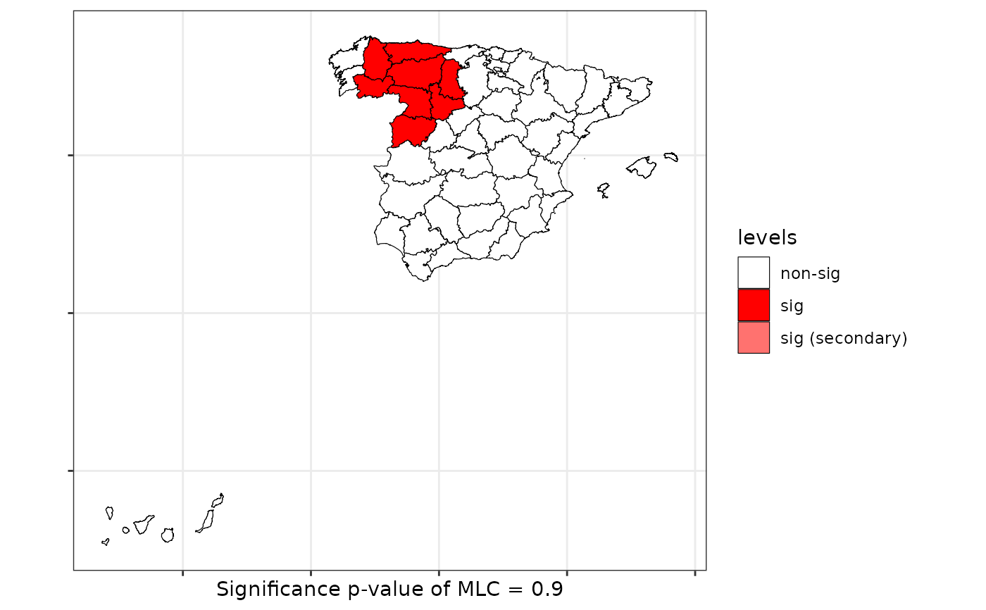
scan <- scan.test(formula = formula, data = provinces_spain, nsim = 99, distr = "multinomial")
print(scan)
#>
#> Scan test. Distribution: multinomial
#>
#> data: Older
#> scan-loglik = 4.2473, p-value = 0.9
#> sample estimates:
#> low middle high Sum
#> cases.expect 2.24 2.88 2.88 8
#> cases.observ 0.00 6.00 2.00 8
#>
plot(scan, sf = provinces_spain)
# Case 2: scan test multinomial
data(provinces_spain)
provinces_spain$Older <- cut(provinces_spain$Older, breaks = c(-Inf,19,22.5,Inf))
levels(provinces_spain$Older) = c("low","middle","high")
formula <- ~ Older
scan <- scan.test(formula = formula, data = provinces_spain, nsim = 99, distr = "multinomial")
print(scan)
#>
#> Scan test. Distribution: multinomial
#>
#> data: Older
#> scan-loglik = 4.2473, p-value = 0.9
#> sample estimates:
#> low middle high Sum
#> cases.expect 2.24 2.88 2.88 8
#> cases.observ 0.00 6.00 2.00 8
#>
plot(scan, sf = provinces_spain)
 # Case 3: scan test multinomial
data(FastFood.sf)
sf::sf_use_s2(FALSE)
formula <- ~ Type
scan <- scan.test(formula = formula, data = FastFood.sf, nsim = 99,
distr = "multinomial", windows="elliptic", nv = 50)
print(scan)
#>
#> Scan test. Distribution: multinomial
#>
#> data: Type
#> scan-loglik = 15.506, p-value < 2.2e-16
#> sample estimates:
#> H P S Sum
#> cases.expect 13.48 14.86 14.66 43
#> cases.observ 16.00 1.00 26.00 43
#>
summary(scan)
#>
#> Summary of data:
#> Distribution....................: multinomial
#> Number of locations.............: 877
#> Total number of cases...........: 877
#> Names of cathegories...........: H P S
#> Total cases per category........: 275 303 299
#> Percent cases per category......: 0.31 0.35 0.34
#>
#> Scan statistic:
#> Total cases in the MLC.........: 43
#> Names of cathegories...........: H P S
#> Observed cases in the MLC......: 13.48 14.86 14.66
#> Expected cases in the MLC......: 16 1 26
#> Value of statistic (loglik ratio)....: 15.5058
#> p-value........................: 0
#>
#> IDs of cluster detect:
#> Location IDs included.....: 68 849 152 499 630 763 827 765 617 600 607 48 58 588 743 843 74 122 750 115 645 61 226 796 876 699 610 597 596 721 751 53 186 659 778 63 106 229 585 738 612 131 208
#>
#>
#> Secondary Scan statistic. Number 1
#> Total cases in secondary cluster......: 16
#> Names of cathegories.................: H P S
#> Percent per category total...........: 0.31 0.35 0.34
#> Percent per category inside cluster..: 0.25 0.5 0.25
#> Value of statisitic (loglik ratio)....: 11.5285
#> p-value.........................: 0.1
#> Location IDs included..................: 677 311 781 128 108 436 551 576 21 374 319 717 561 6 629 547
#>
#>
#> Secondary Scan statistic. Number 2
#> Total cases in secondary cluster......: 7
#> Names of cathegories.................: H P S
#> Percent per category total...........: 0.31 0.35 0.34
#> Percent per category inside cluster..: 0.14 0.29 0.57
#> Value of statisitic (loglik ratio)....: 7.0038
#> p-value.........................: 0.96
#> Location IDs included..................: 158 709 335 801 749 545 856
#>
#>
#> Secondary Scan statistic. Number 3
#> Total cases in secondary cluster......: 17
#> Names of cathegories.................: H P S
#> Percent per category total...........: 0.31 0.35 0.34
#> Percent per category inside cluster..: 0.35 0.35 0.29
#> Value of statisitic (loglik ratio)....: 6.8747
#> p-value.........................: 0.98
#> Location IDs included..................: 521 782 162 643 297 220 267 265 104 530 312 523 783 157 531 848 680
#>
#>
#> Secondary Scan statistic. Number 4
#> Total cases in secondary cluster......: 17
#> Names of cathegories.................: H P S
#> Percent per category total...........: 0.31 0.35 0.34
#> Percent per category inside cluster..: 0.47 0.29 0.24
#> Value of statisitic (loglik ratio)....: 6.7961
#> p-value.........................: 0.98
#> Location IDs included..................: 190 837 555 711 646 216 17 390 742 563 307 4 353 197 254 192 66
#>
#>
#> Secondary Scan statistic. Number 5
#> Total cases in secondary cluster......: 10
#> Names of cathegories.................: H P S
#> Percent per category total...........: 0.31 0.35 0.34
#> Percent per category inside cluster..: 0.4 0.2 0.4
#> Value of statisitic (loglik ratio)....: 6.5951
#> p-value.........................: 0.98
#> Location IDs included..................: 78 365 668 228 170 857 306 708 651 187
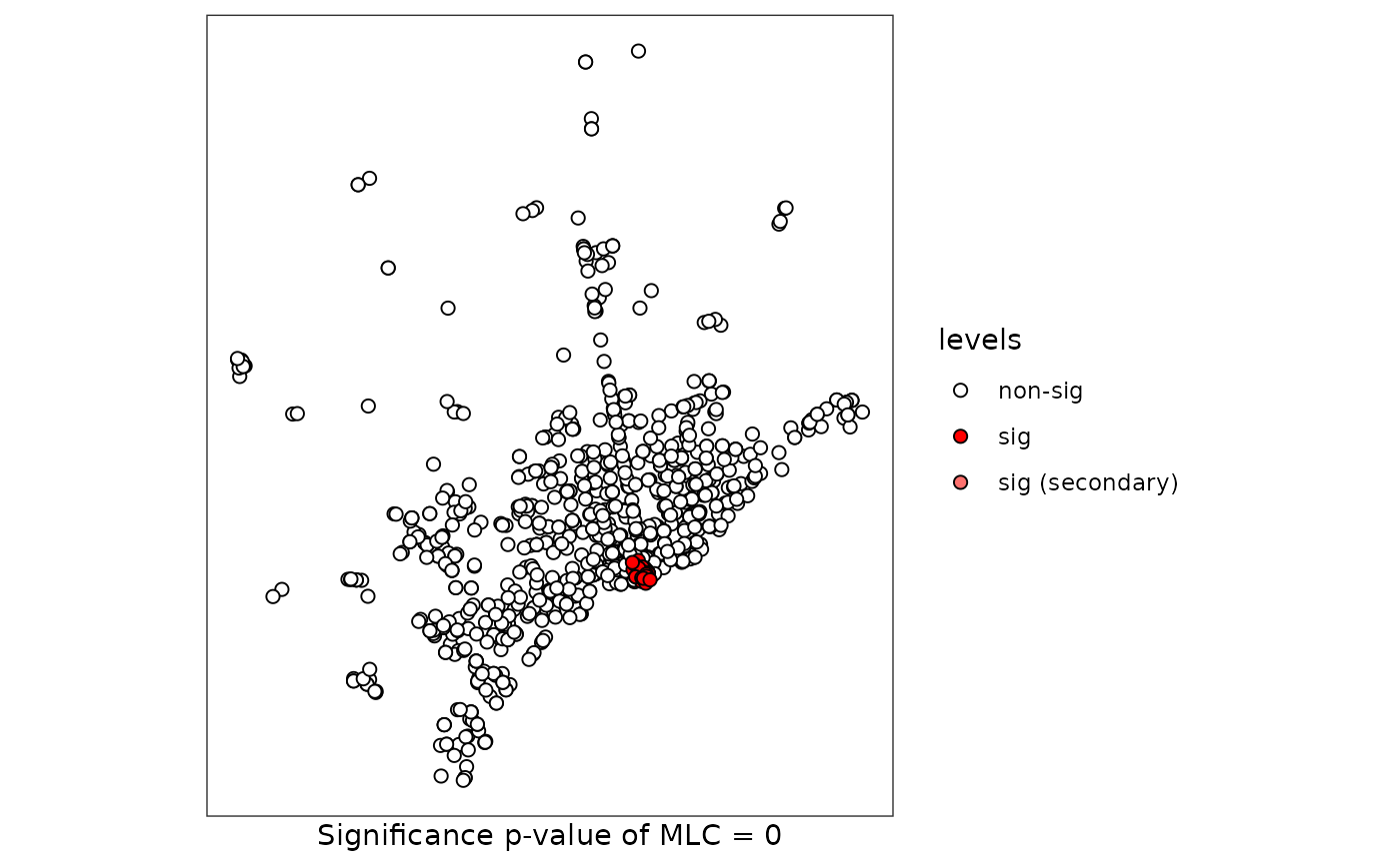
plot(scan, sf = FastFood.sf)
# Case 3: scan test multinomial
data(FastFood.sf)
sf::sf_use_s2(FALSE)
formula <- ~ Type
scan <- scan.test(formula = formula, data = FastFood.sf, nsim = 99,
distr = "multinomial", windows="elliptic", nv = 50)
print(scan)
#>
#> Scan test. Distribution: multinomial
#>
#> data: Type
#> scan-loglik = 15.506, p-value < 2.2e-16
#> sample estimates:
#> H P S Sum
#> cases.expect 13.48 14.86 14.66 43
#> cases.observ 16.00 1.00 26.00 43
#>
summary(scan)
#>
#> Summary of data:
#> Distribution....................: multinomial
#> Number of locations.............: 877
#> Total number of cases...........: 877
#> Names of cathegories...........: H P S
#> Total cases per category........: 275 303 299
#> Percent cases per category......: 0.31 0.35 0.34
#>
#> Scan statistic:
#> Total cases in the MLC.........: 43
#> Names of cathegories...........: H P S
#> Observed cases in the MLC......: 13.48 14.86 14.66
#> Expected cases in the MLC......: 16 1 26
#> Value of statistic (loglik ratio)....: 15.5058
#> p-value........................: 0
#>
#> IDs of cluster detect:
#> Location IDs included.....: 68 849 152 499 630 763 827 765 617 600 607 48 58 588 743 843 74 122 750 115 645 61 226 796 876 699 610 597 596 721 751 53 186 659 778 63 106 229 585 738 612 131 208
#>
#>
#> Secondary Scan statistic. Number 1
#> Total cases in secondary cluster......: 16
#> Names of cathegories.................: H P S
#> Percent per category total...........: 0.31 0.35 0.34
#> Percent per category inside cluster..: 0.25 0.5 0.25
#> Value of statisitic (loglik ratio)....: 11.5285
#> p-value.........................: 0.1
#> Location IDs included..................: 677 311 781 128 108 436 551 576 21 374 319 717 561 6 629 547
#>
#>
#> Secondary Scan statistic. Number 2
#> Total cases in secondary cluster......: 7
#> Names of cathegories.................: H P S
#> Percent per category total...........: 0.31 0.35 0.34
#> Percent per category inside cluster..: 0.14 0.29 0.57
#> Value of statisitic (loglik ratio)....: 7.0038
#> p-value.........................: 0.96
#> Location IDs included..................: 158 709 335 801 749 545 856
#>
#>
#> Secondary Scan statistic. Number 3
#> Total cases in secondary cluster......: 17
#> Names of cathegories.................: H P S
#> Percent per category total...........: 0.31 0.35 0.34
#> Percent per category inside cluster..: 0.35 0.35 0.29
#> Value of statisitic (loglik ratio)....: 6.8747
#> p-value.........................: 0.98
#> Location IDs included..................: 521 782 162 643 297 220 267 265 104 530 312 523 783 157 531 848 680
#>
#>
#> Secondary Scan statistic. Number 4
#> Total cases in secondary cluster......: 17
#> Names of cathegories.................: H P S
#> Percent per category total...........: 0.31 0.35 0.34
#> Percent per category inside cluster..: 0.47 0.29 0.24
#> Value of statisitic (loglik ratio)....: 6.7961
#> p-value.........................: 0.98
#> Location IDs included..................: 190 837 555 711 646 216 17 390 742 563 307 4 353 197 254 192 66
#>
#>
#> Secondary Scan statistic. Number 5
#> Total cases in secondary cluster......: 10
#> Names of cathegories.................: H P S
#> Percent per category total...........: 0.31 0.35 0.34
#> Percent per category inside cluster..: 0.4 0.2 0.4
#> Value of statisitic (loglik ratio)....: 6.5951
#> p-value.........................: 0.98
#> Location IDs included..................: 78 365 668 228 170 857 306 708 651 187
plot(scan, sf = FastFood.sf)
 # Case 4: DGP two categories
N <- 150
cx <- runif(N)
cy <- runif(N)
listw <- spdep::knearneigh(cbind(cx,cy), k = 10)
p <- c(1/2,1/2)
rho <- 0.5
fx <- dgp.spq(p = p, listw = listw, rho = rho)
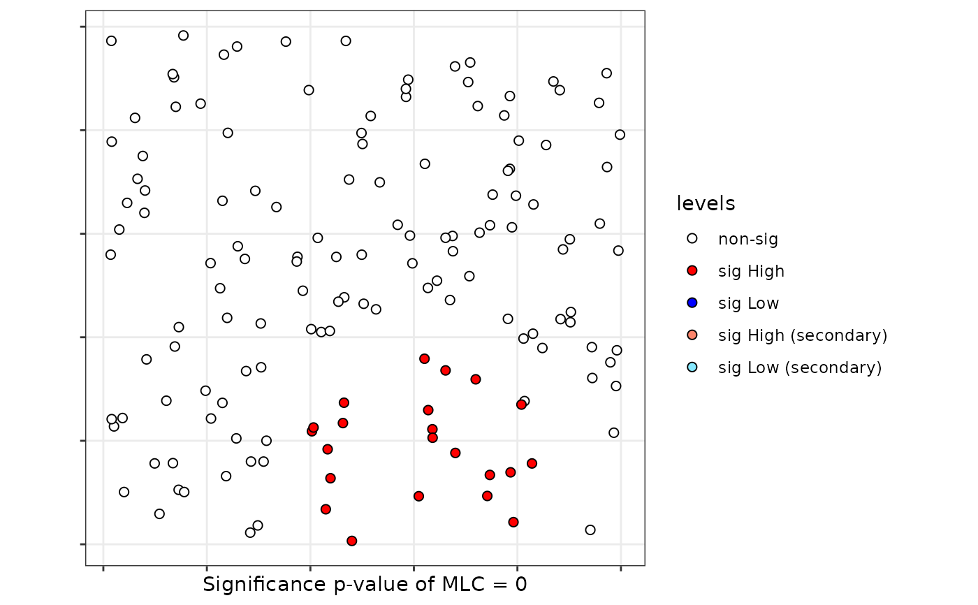
scan <- scan.test(fx = fx, nsim = 99, case = "A", nv = 50, coor = cbind(cx,cy),
distr = "bernoulli",windows="circular")
print(scan)
#>
#> Scan test. Distribution: bernoulli
#>
#> data: fx
#> scan-loglik = 4.8102, p-value = 0.51
#> alternative hypothesis: High
#> sample estimates:
#>
#> Total observations in the MLC = 44.0
#> Expected cases in the MLC = 21.5
#> Observed cases in the MLC = 30.0
#>
plot(scan)
# Case 4: DGP two categories
N <- 150
cx <- runif(N)
cy <- runif(N)
listw <- spdep::knearneigh(cbind(cx,cy), k = 10)
p <- c(1/2,1/2)
rho <- 0.5
fx <- dgp.spq(p = p, listw = listw, rho = rho)
scan <- scan.test(fx = fx, nsim = 99, case = "A", nv = 50, coor = cbind(cx,cy),
distr = "bernoulli",windows="circular")
print(scan)
#>
#> Scan test. Distribution: bernoulli
#>
#> data: fx
#> scan-loglik = 4.8102, p-value = 0.51
#> alternative hypothesis: High
#> sample estimates:
#>
#> Total observations in the MLC = 44.0
#> Expected cases in the MLC = 21.5
#> Observed cases in the MLC = 30.0
#>
plot(scan)
 # Case 5: DGP three categories
N <- 200
cx <- runif(N)
cy <- runif(N)
listw <- spdep::knearneigh(cbind(cx,cy), k = 10)
p <- c(1/3,1/3,1/3)
rho <- 0.5
fx <- dgp.spq(p = p, listw = listw, rho = rho)
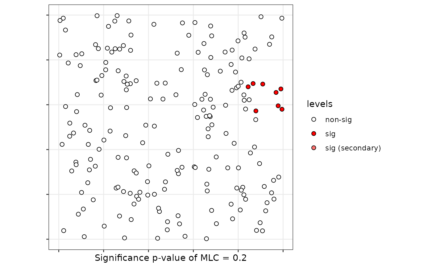
scan <- scan.test(fx = fx, nsim = 19, coor = cbind(cx,cy), nv = 30,
distr = "multinomial", windows = "elliptic")
print(scan)
#>
#> Scan test. Distribution: multinomial
#>
#> data: fx
#> scan-loglik = 14.29, p-value < 2.2e-16
#> sample estimates:
#> A B C Sum
#> cases.expect 8.04 7.92 8.04 24
#> cases.observ 0.00 6.00 18.00 24
#>
plot(scan)
# Case 5: DGP three categories
N <- 200
cx <- runif(N)
cy <- runif(N)
listw <- spdep::knearneigh(cbind(cx,cy), k = 10)
p <- c(1/3,1/3,1/3)
rho <- 0.5
fx <- dgp.spq(p = p, listw = listw, rho = rho)
scan <- scan.test(fx = fx, nsim = 19, coor = cbind(cx,cy), nv = 30,
distr = "multinomial", windows = "elliptic")
print(scan)
#>
#> Scan test. Distribution: multinomial
#>
#> data: fx
#> scan-loglik = 14.29, p-value < 2.2e-16
#> sample estimates:
#> A B C Sum
#> cases.expect 8.04 7.92 8.04 24
#> cases.observ 0.00 6.00 18.00 24
#>
plot(scan)
 # Case 6: Flexible windows
data(provinces_spain)
sf::sf_use_s2(FALSE)
provinces_spain$Mal2Fml <- factor(provinces_spain$Mal2Fml > 100)
#> Warning: ‘>’ not meaningful for factors
levels(provinces_spain$Mal2Fml) = c("men","woman")
formula <- ~ Mal2Fml
listw <- spdep::poly2nb(provinces_spain, queen = FALSE)
#> although coordinates are longitude/latitude, st_intersects assumes that they
#> are planar
#> Warning: some observations have no neighbours;
#> if this seems unexpected, try increasing the snap argument.
#> Warning: neighbour object has 4 sub-graphs;
#> if this sub-graph count seems unexpected, try increasing the snap argument.
scan <- scan.test(formula = formula, data = provinces_spain, case="men", listw = listw, nv = 6,
nsim = 99, distr = "bernoulli", windows = "flexible")
#> Error in scan.test(formula = formula, data = provinces_spain, case = "men", listw = listw, nv = 6, nsim = 99, distr = "bernoulli", windows = "flexible"): The factor mut be have 2 levels for bernoulli
print(scan)
#>
#> Scan test. Distribution: multinomial
#>
#> data: fx
#> scan-loglik = 14.29, p-value < 2.2e-16
#> sample estimates:
#> A B C Sum
#> cases.expect 8.04 7.92 8.04 24
#> cases.observ 0.00 6.00 18.00 24
#>
summary(scan)
#>
#> Summary of data:
#> Distribution....................: multinomial
#> Number of locations.............: 200
#> Total number of cases...........: 200
#> Names of cathegories...........: A B C
#> Total cases per category........: 67 66 67
#> Percent cases per category......: 0.34 0.33 0.34
#>
#> Scan statistic:
#> Total cases in the MLC.........: 24
#> Names of cathegories...........: A B C
#> Observed cases in the MLC......: 8.04 7.92 8.04
#> Expected cases in the MLC......: 0 6 18
#> Value of statistic (loglik ratio)....: 14.2905
#> p-value........................: 0
#>
#> IDs of cluster detect:
#> Location IDs included.....: 76 27 46 29 185 190 167 13 52 195 122 79 70 2 62 35 32 133 103 77 9 162 115 75
#>
#>
#> Secondary Scan statistic. Number 1
#> Total cases in secondary cluster......: 26
#> Names of cathegories.................: A B C
#> Percent per category total...........: 0.34 0.33 0.34
#> Percent per category inside cluster..: 0.42 0.35 0.23
#> Value of statisitic (loglik ratio)....: 7.4166
#> p-value.........................: 0.65
#> Location IDs included..................: 148 188 80 42 184 200 54 98 48 8 40 124 128 153 89 114 39 129 99 142 189 56 125 38 176 108
#>
#>
#> Secondary Scan statistic. Number 2
#> Total cases in secondary cluster......: 13
#> Names of cathegories.................: A B C
#> Percent per category total...........: 0.34 0.33 0.34
#> Percent per category inside cluster..: 0.23 0.31 0.46
#> Value of statisitic (loglik ratio)....: 5.7996
#> p-value.........................: 0.95
#> Location IDs included..................: 112 149 154 130 137 84 140 187 145 194 174 199 7
#>
#>
#> Secondary Scan statistic. Number 3
#> Total cases in secondary cluster......: 8
#> Names of cathegories.................: A B C
#> Percent per category total...........: 0.34 0.33 0.34
#> Percent per category inside cluster..: 0.38 0.25 0.38
#> Value of statisitic (loglik ratio)....: 5.0397
#> p-value.........................: 0.95
#> Location IDs included..................: 14 109 175 30 107 143 152 74
#>
#>
#> Secondary Scan statistic. Number 4
#> Total cases in secondary cluster......: 8
#> Names of cathegories.................: A B C
#> Percent per category total...........: 0.34 0.33 0.34
#> Percent per category inside cluster..: 0.5 0.25 0.25
#> Value of statisitic (loglik ratio)....: 4.9452
#> p-value.........................: 0.95
#> Location IDs included..................: 110 150 139 161 102 104 147 111
#>
#>
#> Secondary Scan statistic. Number 5
#> Total cases in secondary cluster......: 5
#> Names of cathegories.................: A B C
#> Percent per category total...........: 0.34 0.33 0.34
#> Percent per category inside cluster..: 0.4 0.6 0
#> Value of statisitic (loglik ratio)....: 4.5181
#> p-value.........................: 0.95
#> Location IDs included..................: 51 141 1 65 34
plot(scan, sf = provinces_spain)
# Case 6: Flexible windows
data(provinces_spain)
sf::sf_use_s2(FALSE)
provinces_spain$Mal2Fml <- factor(provinces_spain$Mal2Fml > 100)
#> Warning: ‘>’ not meaningful for factors
levels(provinces_spain$Mal2Fml) = c("men","woman")
formula <- ~ Mal2Fml
listw <- spdep::poly2nb(provinces_spain, queen = FALSE)
#> although coordinates are longitude/latitude, st_intersects assumes that they
#> are planar
#> Warning: some observations have no neighbours;
#> if this seems unexpected, try increasing the snap argument.
#> Warning: neighbour object has 4 sub-graphs;
#> if this sub-graph count seems unexpected, try increasing the snap argument.
scan <- scan.test(formula = formula, data = provinces_spain, case="men", listw = listw, nv = 6,
nsim = 99, distr = "bernoulli", windows = "flexible")
#> Error in scan.test(formula = formula, data = provinces_spain, case = "men", listw = listw, nv = 6, nsim = 99, distr = "bernoulli", windows = "flexible"): The factor mut be have 2 levels for bernoulli
print(scan)
#>
#> Scan test. Distribution: multinomial
#>
#> data: fx
#> scan-loglik = 14.29, p-value < 2.2e-16
#> sample estimates:
#> A B C Sum
#> cases.expect 8.04 7.92 8.04 24
#> cases.observ 0.00 6.00 18.00 24
#>
summary(scan)
#>
#> Summary of data:
#> Distribution....................: multinomial
#> Number of locations.............: 200
#> Total number of cases...........: 200
#> Names of cathegories...........: A B C
#> Total cases per category........: 67 66 67
#> Percent cases per category......: 0.34 0.33 0.34
#>
#> Scan statistic:
#> Total cases in the MLC.........: 24
#> Names of cathegories...........: A B C
#> Observed cases in the MLC......: 8.04 7.92 8.04
#> Expected cases in the MLC......: 0 6 18
#> Value of statistic (loglik ratio)....: 14.2905
#> p-value........................: 0
#>
#> IDs of cluster detect:
#> Location IDs included.....: 76 27 46 29 185 190 167 13 52 195 122 79 70 2 62 35 32 133 103 77 9 162 115 75
#>
#>
#> Secondary Scan statistic. Number 1
#> Total cases in secondary cluster......: 26
#> Names of cathegories.................: A B C
#> Percent per category total...........: 0.34 0.33 0.34
#> Percent per category inside cluster..: 0.42 0.35 0.23
#> Value of statisitic (loglik ratio)....: 7.4166
#> p-value.........................: 0.65
#> Location IDs included..................: 148 188 80 42 184 200 54 98 48 8 40 124 128 153 89 114 39 129 99 142 189 56 125 38 176 108
#>
#>
#> Secondary Scan statistic. Number 2
#> Total cases in secondary cluster......: 13
#> Names of cathegories.................: A B C
#> Percent per category total...........: 0.34 0.33 0.34
#> Percent per category inside cluster..: 0.23 0.31 0.46
#> Value of statisitic (loglik ratio)....: 5.7996
#> p-value.........................: 0.95
#> Location IDs included..................: 112 149 154 130 137 84 140 187 145 194 174 199 7
#>
#>
#> Secondary Scan statistic. Number 3
#> Total cases in secondary cluster......: 8
#> Names of cathegories.................: A B C
#> Percent per category total...........: 0.34 0.33 0.34
#> Percent per category inside cluster..: 0.38 0.25 0.38
#> Value of statisitic (loglik ratio)....: 5.0397
#> p-value.........................: 0.95
#> Location IDs included..................: 14 109 175 30 107 143 152 74
#>
#>
#> Secondary Scan statistic. Number 4
#> Total cases in secondary cluster......: 8
#> Names of cathegories.................: A B C
#> Percent per category total...........: 0.34 0.33 0.34
#> Percent per category inside cluster..: 0.5 0.25 0.25
#> Value of statisitic (loglik ratio)....: 4.9452
#> p-value.........................: 0.95
#> Location IDs included..................: 110 150 139 161 102 104 147 111
#>
#>
#> Secondary Scan statistic. Number 5
#> Total cases in secondary cluster......: 5
#> Names of cathegories.................: A B C
#> Percent per category total...........: 0.34 0.33 0.34
#> Percent per category inside cluster..: 0.4 0.6 0
#> Value of statisitic (loglik ratio)....: 4.5181
#> p-value.........................: 0.95
#> Location IDs included..................: 51 141 1 65 34
plot(scan, sf = provinces_spain)
 # }
# }